


A Fusion Approach of Reinforcement Learning and Traffic Engineering in Multiple Traffic Signal Control
- Traffic Signal Control
- Reinforcement Learning
- Traffic Engineering
- Subarea Control
- AI Technology
The quality of traffic signal control is directly linked to such social issues as traffic jams and environmental issues. In the past, skilled engineers have maintained and improved this quality. For signal control, we need to adjust the signals with neighboring ones. The difficulty in optimizing signal control lies in coordinating signals with their neighbor signals. We control multiple signals together in sub-area units based on traffic engineering. In recent years, with the development of artificial intelligence (AI), many methods using reinforcement learning (RL) for sub-area control have been proposed. However, many of these methods do not rely on traditional traffic engineering. They use AI approaches like multi-agent reinforcement learning (MARL). Therefore, even if such measures as delay time improve, we find difficult to say that these methods are ready to be used for real-world traffic signal control yet.
In this study, we first investigate how current RL approaches relate to important traffic engineering parameters, such as cycle, split, and offset. Additionally, we propose an implementable signal control method by combining reinforcement learning with traditional traffic engineering. Specifically, we introduce two constraints—coordination constraints and time constraints—derived from traffic engineering. Here we show, in traditional reinforcement learning, the cycle and split significantly vary each time, making it impractical. Additionally, with time constraints, we reduced the delay time, an evaluation metric, from 116 seconds/car to 95 seconds/car, and CO2 emissions decreased by 18%. On the other hand, the coordination constraints did not contribute to reducing delay times or CO2 emissions. This result demonstrates the potential of integrating traffic engineering with RL to develop effective signal control methods.
This paper targets traffic signal control in Japan, where vehicles drive on the left side of the road.
1. Introduction
Ever-worsening traffic congestion is costing the modern world massive time losses and economic burdens, as well as air pollution and other environmental problems. For example, the Ministry of Land, Infrastructure and Transport points out in a document1) that traffic congestion has cost the nation approximately 6.1 billion hours per year. In response, the Japanese government has included the creating of sustainable, livable communities and digitally transforming and decarbonizing the infrastructure sector in its key policy target list in the Fifth Priority Plan for Social Infrastructure Development. In this plan, the National Police Agency encourages efforts towards efficient road transportation and enhanced road safety2).
The key to smooth road traffic flow lies in road traffic signal control (hereinafter “signal control”) in a road traffic control system. The current practice is for experienced engineers to survey candidate sites and draft traffic engineering-based proposals, followed by pilot and final implementation. However, the recent aging society with fewer children, along with the resulting shortage of experienced engineers and surge in labor costs, has led to proposals for signal control using machine learning and especially reinforcement learning. We have also reported the results of an investigation on a reinforcement learning-based control method for single signals3).
Incidentally, traffic lights are not individually controlled. The common practice is to use centralized control of multiple traffic lights. A set of such collectively controlled traffic lights constitutes a unit called a sub-area. In actual practice, control parameters are set for each sub-area. Papers already exist on reinforcement learning for collective control of multiple signals in sub-areas4,5). Recent mainstream studies aim to achieve optimization using such machine learning techniques as multi-agent reinforcement learning (MARL) and graph convolutional networks (GCN). As a result, delay times and other performance indices have improved. However, it cannot yet be said that the applicability of these ML techniques to actual signal control has been sufficiently considered. It remains particularly unclear what outputs reinforcement learning-based conventional methods provide for cycle length, splits, and offsets, the three signal control indices based on today’s traffic engineering. Neither is it clear whether these methods would be practically functional for human drivers in actual traffic flows compared with the current signal control.
To address these questions, this paper first, in section 2, outlines the current reinforcement learning-based control and introduces three important traffic engineering parameters: cycle length, split, and offset. Section 3 proposes a signal control approach that integrates constraints from conventional traffic engineering into RL-based control. Section 4 presents the results from a simulation verifying the effectiveness of the proposed signal control.
2. Conventional technologies and prior studies
2.1 Signal control based on traffic engineering
Each of the green, yellow, and red indications on typical traffic lights is called a phase. This paper regards phases with a right-turn arrow on a red signal as green phases. From the perspective of traffic engineering, what matters the most to control multiple signals in sub-areas with groups of collectively controlled traffic lights are the three parameters known as cycle length, offset, and split (Fig. 1). For detailed calculations for these parameters, refer to Planning and Design of At-Grade Intersections6), a design handbook published by the Japan Society of Traffic Engineers (JSTE).
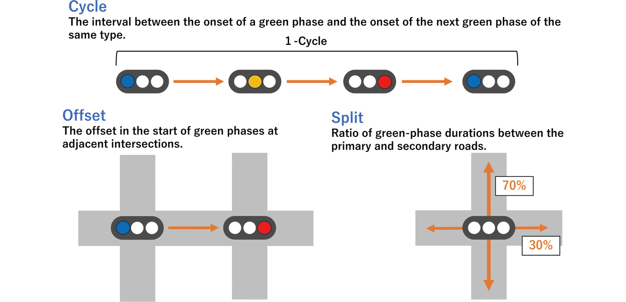
The term “cycle length” refers to the time it takes for a signal to return to its current phase. A cycle length is calculated using the loss time L, which consists of practically vehicle-impassable durations within a single cycle, such as the yellow and red phases, and the flow ratio λ, the ratio of actual traffic volume to theoretical intersection capacity. First of all, a cycle length below the theoretical minimum value yields an intersection capacity short of the traffic volume, which always results in traffic congestion. In addition, with a cycle length close to Cmin, even a slight increase in the number of vehicles can cause traffic congestion. Hence, some allowance should be made. An example of a cycle length with this allowance is F. V. Webster’s proposed value Cp, which is optimized under the assumption that vehicle emergences follow a Poisson distribution. Another example is the JSTE’s proposed value with an estimated allowance of 11%. For their calculation, the following equations are used:
In actual field practice, a cycle length is usually set in 10-second increments with reference to the Cp or value. On the other hand, an unreasonably long cycle length irritates drivers and can lead to risks, such as forceful drive-through or traffic signal violations. Hence, most cycle lengths are set within 180 seconds. A unified cycle length should desirably be used across the sub-area to ensure a uniform offset for each cycle. Usually, a unified cycle length is referenced to the cycle length of the longest intersection.
An offset is a parameter that inserts a time lag between the phase start timings of two adjacent intersections. Setting an appropriate offset enables vehicles to proceed smoothly from one intersection to another, reducing traffic congestion in urban areas and on arterial roads.
Offsets actually used primarily fall into the following three types:
- Simultaneous offset: The offset of each signal is set to 0 to trigger a simultaneous green phase on the major road.
- Alternate offset: The offset of each signal is set to exactly half the cycle length to trigger alternating green phases on the major road.
- Preferential offset: Adjusted so that a major-road green phase starts at a signalized intersection exactly when the front-lead vehicles on the inbound (or outbound) lanes arrive there after departing a green light at the adjacent intersection and then traveling at the limit speed. Adopted when inbound and outbound traffic demand differs considerably.
From these offset types, an appropriate one is selected, depending on the current traffic situation.
The term “split” refers to the ratio of the green light time allocated to each direction of travel. A longer green signal time is set for a direction with a higher vehicle flow rate and vice versa to reduce overall wait time or improve intersection throughput.
Signal control engineers consider the traffic volume, intersection geometry, and intersection spacing in each sub-area to appropriately adjust and set the signal control parameters (cycle length, split, and offset).
2.2 Reinforcement Learning
Reinforcement Learning (hereinafter “RL”) is a framework where an agent learns an optimal strategy (or “policy”) through trial and error while interacting with an environment. The agent observes the environment’s state at each time step and selects an action based on the state obtained. As a result of the action, the environment changes, and the agent receives feedback as a reward. A reward is a numerical indicator that shows the desirability of the action. The agent continues learning to maximize the cumulative reward (return).
As regards the theoretical background, an RL problem is formulated as a Markov decision process (MDP). An MDP integrates the four elements of state, action, reward, and transition probability into an environment model. This framework provides a foundation for the existence of an optimal policy for an agent to maximize future rewards. It also serves as a basis for deriving the optimality conditions for that purpose from the Bellman equation. Thanks to this framework, many RL algorithms have theoretical validity and demonstrate their effectiveness in actual applications.
To explain the framework of RL, let us define the following symbols:
- S: A universal set of states that an agent can take. Each element is represented by s.
- A: A universal set of actions that an agent can take. Each element is represented by a.
- P(s′ | s,a): Known as the state transition probability, which is the probability of the current state s ∈ S and action a ∈ A determining the subsequent state s′ ∈ S.
- r (s,a): Known as immediate reward, which is the reward for action a taken in state s.
- γ ∈[0,1] : Known as the discount factor, which is a parameter that determines how much future rewards should matter. A discount factor closer to zero emphasizes shortterm rewards, while one closer to one emphasizes long-term rewards.
- π: Known as policy, which is a rule that dictates what action an agent should take, depending on the current state. Especially when given as π (a | s), the policy denotes the probability of taking action a in state s. An optimal policy is given as π*.
The agent’s objective is to maximize the expected cumulative reward. The cumulative reward Gt at time t is defined as follows:
Then, let us introduce a quantitative indicator that shows how good a state or an action is. The action-value function Qπ(s,a) for when a policy π is complied with is a value function for when action a is selected in state s. This function is defined as follows:
This equation represents the expected cumulative reward for the action a selected in the state s, followed by acting in accordance with the policy π. Therefore, when an optimal action-value function Q*(s,a) is already obtained, the agent can earn the highest expected cumulative reward by selecting action a with the highest action value every time. Therefore, the optimal policy to be obtained is defined as π*(s) = argmaxaQ*(s,a).
However, few cases exist in which an action-value function can be analytically calculated. Hence, Q-Learning was proposed as a method for sequentially deriving an optimal action-value function. Q-Learning takes advantage of how well the action-value function cab be rewritten into the following recursive form:
to sequentially update and optimize the action-value function by means of the following formula:
where α is the learning rate and the argument means taking into account the maximum action value in the next state s′ to learn an optimal policy. To be sure, Q-Learning has relatively low computational complexity with fewer states and actions. However, its computational complexity increases quickly with the number of states and actions. As a result, individual estimations become harder to make. To address this issue, the Deep Q-Network (DQN)7) uses neural networks for the Q-value estimation. This paper also adopts this RL algorithm.
2.3 RL-based signal control
Various methods have been proposed for RL-based signal control. In the earliest days, back in the 2000s, Wiering and Abdulhai used Q-learning for signal control8,9). Entering the 2010s, Li introduced DQN to start deep learning-based signal control10).
Moreover, Sato11) proposed a method that uses not only the mere flow-rate and signal information but also aerial-view images as inputs. Meanwhile, Han12) introduced queuing estimation models into DQN. However, Sato and Han limited their investigations to single signals. By contrast, this paper compares three different types of methods, single-agent, information-exchange multi-agent, and independent multi-agent types, to consider an RL-based multi-signal determination method.
The single-agent type controls the whole sub-area with a single RL AI agent. The agent receives information on the entire sub-area as input, making overall optimization more achievable. On the other hand, the agent faces an exponential increase in the number of states and actions as the number of traffic lights grows. Above all, the sub-area assigned to us had up to 16 signals, which translates into a total of 216 = 65,536 different actions, an unrealistically large quantity to control with RL. In addition, each signal state varies across sub-areas, each with a different number of signals or geometry, requiring individual customization for each sub-area at the expense of scalability. Kuwahara13) reported on single-agent-based RL, noting that even a sub-area with two signals requires an extremely large number of learning iterations.
The information-exchange multi-agent type assigns one agent to each signal. Each agent exchanges specific kinds of information, such as traffic volume or the current signal phase, with its peers in the surroundings. This information serves as the ego-agent state input for RL-based control. Overseas research reports abound on this system type. Wei14) proposed a method to incorporate the states of intersections in the surroundings as intersection input information. Nishi15) and Wang16) proposed methods to exchange information using a Graph Neural Network (GNN). Compared with single-agent types, these methods better address the challenge posed by the number of actions but still require individual customization for each sub-area and offer limited scalability.
The independent multi-agent type assigns one agent to each signal and controls using only ego-agent information. Not only can this method achieve individual optimization, but it also allows the iterative reuse of RL agents. Thus, the method offers high scalability as one of its advantages. On the other hand, each agent accepts information as an entry only from the surroundings of its ego intersection. Thus, this method has the drawback of achieving individual rather than overall optimization.
3. Fusion algorithm between traffic engineering and RL
This section proposes a control algorithm that fuses traffic engineering with independent multi-agent RL, one of the three RL types presented in section 2. The first reason is that the information-exchange multi-agent type, which has many variants in the literature, requires individual customization for each sub-area and increases the person-hours spent on signal control considerations, contrary to the intended goal. The second reason is the problem with other efforts underway to achieve overall optimization using advanced AI technologies, such as MARL and GNNs. Such complex AI technologies are too troublesome for field engineers to understand and operate. In the event of anomalies, they provide low explainability.
The independent multi-agent type must overcome two challenges for implementation in actual signal control. The first challenge is that adjacent signals are poorly coordinated because of individual optimal control with each signal’s close-proximity surroundings being the sole consideration. Hence, for example, at a signalized intersection, the signals turn red immediately after the arrival of vehicles that departed upon a green light at the adjacent intersections, thereby achieving individual, but not necessarily overall, optimization. The second challenge is that the RL evaluation function may not always be optimal. In particular, DQN uses deep learning and, as such, may take extreme actions due to overfitting/error divergence or gradient disappearance/explosion. For example, DQN may truncate a supposedly 60-second-long major-road green phase after 3 seconds. Conversely, DQN may give 60 seconds to a minor-road right turn that can be handled within 3 seconds.
To address these two challenges, we build on traffic engineering and propose imposing the constraints listed below based on the independent multi-agent type.
For the first challenge, constraints tailored to the phases of the adjacent signals are imposed to solve it. At the most congested intersection, even the slightest shift in a signal phase would cause a significant impact. On the other hand, at a low-traffic-volume intersection, a certain amount of signal-phase shifting would have only a minor impact. Hence, we use unconstrained control for the center signals at the most congested intersection, while subjecting the adjacent signals (dependent signals) to a limited set of constraints dependent on the center-signal phase status. More specifically, we imposed the following constraints to ensure that a simultaneous offset would be obtained:
- If the center signals are in the major-road green phase, the dependent signals must not proceed to the next phase until the major-road green phase ends.
- If the center signals are in any of the phases other than the major-road green phase, the dependent signals may proceed to the next green phase before the center signals but must not proceed to the subsequent yellow and red phases. Otherwise, the offset type would change from simultaneous to alternate.
- After the center signals the transition to the next phase, the dependent signals must follow within 6 seconds, which is the sum of the yellow signal time of 3 seconds and the minimum green signal time of 3 seconds. Failure to comply will result in a loss of synchronization with the center signal two phases ahead of the dependent ones.
- To establish an alternate offset, interchange the center signalsʼ major- and minor-road conditions.
These constraints are referred to below as “coordination constraints.”
For the second challenge, minimum and maximum time limits in seconds must be set for each phase type to avoid extremes, such as dangerously short times or unreasonably long stops. More specifically, we adopted the following settings:
- Minimum seconds: The number of seconds for each phase type in a Cmin-second cycle rounded up to the nearest 10-second increment. Determined on the basis of the split calculated from the traffic volume ratio.
- Maximum seconds: The number of seconds for each phase type in a 180-second cycle. Determined on the basis of the split calculated from the traffic volume ratio.
These settings ensure that each signal’s phase time falls within a range deemed appropriate from a traffic engineering perspective. These settings are referred to below as “time constraints.”
4. Experimental method and results
4.1 Experimental conditions and evaluation method
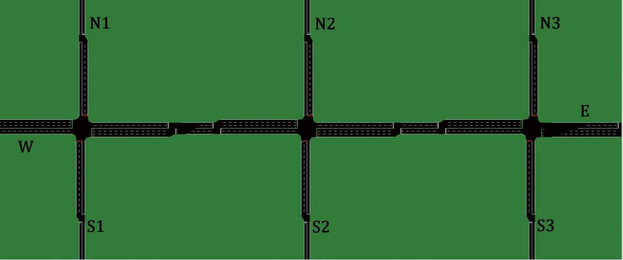
Among the sub-areas of the various geometries, the geometrically most common ones are found along straight-line sections of major roads. The target of experimental interest in this paper was a sub-area of this geometry comprising three signals along a straight-line section of an arterial road. The simulation environment used was the Simulation of Urban MObility (SUMO)17). As in Fig. 2, the ends of the relevant road sections were named W, N1, N2, N3, E, S3, S2, and S1 clockwise from left to right. The major road (W-E) was a two-lane-per-side road with a speed limit of 60 km/h and included a pair of approximately 75 m long right-turn lanes at each intersection. The three minor roads (N1-S1, N2-S2, and N3-S3) were one-lane-per-side roads with a speed limit of 50 km/h, and each included a pair of approximately 75 m long right-turn lanes at their respective intersections. Each adjacent intersection was spaced 250 m center to center from the central intersection.
The comparative reference used was the conventional fixed-time control and calculated in accordance with Planning and Design of At-Grade Intersections. Fixed-time control is the most basic form of control in which phases always progress for a fixed time regardless of the situation. Table 1 below shows the phase-time settings for each fixed-time-controlled signal. The cycle length was set to 80 seconds as calculated from the flow ratio, λ = 0.74, for the traffic volumes in Table 3 with reference to F. V. Webster’s proposed value of Cp = 88 and the Japan Society of Traffic Engineers’ recommended value of = 68. The phase splits were determined to match the traffic volume ratios. With no traffic-volume bias assumed in this experiment, all signals were operated with simultaneous offsets.
| Signal | Cycle length | Major-road green | Major-road right turn | Minor-road green | Minor-road right turn |
|---|---|---|---|---|---|
| Central intersection | 80 s | 28 | 6 | 25 | 3 |
| Left/right intersection | 80 s | 33 | 5 | 21 | 3 |
Table 2 lists the RL time-constraint parameters (in seconds). The minimum and maximum cycle lengths were set to 60 and 180 seconds, respectively, and the phase times were again based on the splits specified to match the traffic volume ratios.
| Signal | Cycle length | Major-road green | Major-road right turn | Minor-road green | Minor-road right turn |
|---|---|---|---|---|---|
| Central intersection | Min. (60 s) |
19 | 3 | 18 | 3 |
| Max. (180 s) |
69 | 18 | 64 | 11 | |
| Left/right intersection | Min. (60 s) |
23 | 3 | 15 | 3 |
| Max. (180 s) |
81 | 17 | 53 | 11 |
For RL training and inference, we used the DQN provided by SUMO-RL18). The state s input to the DQN consisted of the current signal phase, the vehicle density per lane, and the queued vehicle density per lane. Action a was an either-or selection: whether to switch to the next phase or continue the current phase. If an RL-derived action failed to meet any of the constraint conditions presented in section 3, the other action option meeting the constraint was selected and executed. For example, assume that the RL algorithm selected switching to the next phase as the action, even though the minimum required number of seconds was not met. In this case, the signal would not switch. Conversely, if the maximum number of seconds were reached, the signal would switch regardless of the RL-selected action. The reward r was the amount of change in the delay time resulting from taking an action. For training, the flow rate pattern P1 below was used to run 1,500,000 steps.
The following three flow rate patterns were used to verify the traffic flow rate from 0 seconds to 10,800 seconds (3 hours):
- P1: Traffic volume specified in Table 3 (flow ratio λ = 0.74 at the center signals)
- P2: Same as P1, except with the major-road traffic volume increasing only for the period from 3,600 seconds to 7,200 seconds (flow ratio λ = 0.82)
- P3: Same as P1, except with the major-road traffic volume decreasing only for the period from 3,600 seconds to 7,200 seconds (flow ratio λ = 0.66)
| From/To [Vehs/hr] |
W | N1 | N2 | N3 | S1 | S2 | S3 | E |
|---|---|---|---|---|---|---|---|---|
| W | \ | 120 | 150 | 120 | 120 | 150 | 120 | 560 (P1) 840 (P2) 280 (P3) |
| N1 | 80 | \ | 0 | 0 | 320 | 0 | 0 | 80 |
| N2 | 100 | 0 | \ | 0 | 0 | 400 | 0 | 100 |
| N3 | 80 | 0 | 0 | \ | 0 | 0 | 320 | 80 |
| S1 | 80 | 320 | 0 | 0 | \ | 0 | 0 | 80 |
| S2 | 100 | 0 | 400 | 0 | 0 | \ | 0 | 100 |
| S3 | 80 | 0 | 0 | 320 | 0 | 0 | \ | 80 |
| E | 560 (P1) 840 (P2) 280 (P3) |
120 | 150 | 120 | 120 | 150 | 120 | \ |
We assumed that vehicles emerged not at uniform intervals but at random intervals that varied from vehicle to vehicle. Then, the emergence of vehicles followed a Poisson distribution with the expected value per unit time equal to the set number of vehicles. For instance, assume an hourly traffic flow of 360 vehicles/hour. Then, it follows not that one vehicle emerges exactly at regular intervals of 10 seconds but that it emerges according to the Poisson distribution on a second-to-second basis. In this case, no vehicle emerges with a probability of 90.4%, one vehicle emerges with a probability of 9%, two vehicles simultaneously emerge with a probability of 0.5%, and three or more vehicles simultaneously emerge with a probability of 0.01% (the total does not add up to 100% because of rounding).
The evaluation method used was the sum of the pre-departure lag (wait) time and the post-departure lag (delay) time per vehicle. In SUMO, when one or more vehicles are already at the point of departure and prevent new vehicles from leaving, another departure attempt is made with a one-second delay. This type of standby time spent unable to depart is called the “departure wait time.” Meanwhile, “delay time” refers to the difference between the actual travel time from the departure end to the destination end and the theoretical constant-speed travel time required to cover the same distance at the limit speed. This value represents the lag time as a negative effect of signal control.
Moreover, we calculated CO2 emissions per vehicle as a reference index. For the CO2 emissions calculation, we used the four-passenger gasoline car model specified in the Handbook of Emission Factors for Road Transport, Version 3, as the standard calculation method for SUMO. The results may be biased by the stochastic emergence of vehicles under the Poisson distribution. Therefore, we ran 50 trials while changing the seed value to the random number generator.
4.2 Experimental results
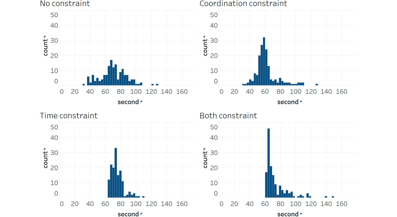
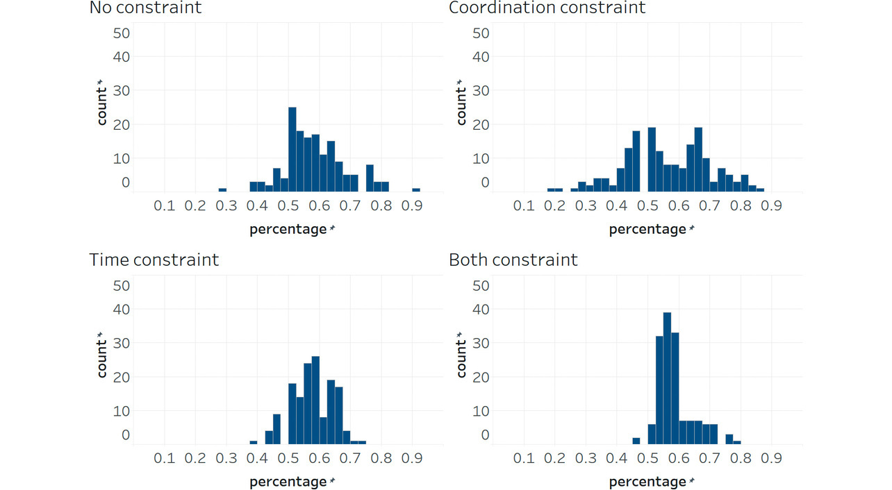
First, for unconstrained RL, Fig. 3 shows cycle-length and split distribution charts for the right intersection and an offset distribution chart between the central and right intersections from a simulation with a random-number seed of 1. (The charts given below of cycle length, splits, and offsets all show values simulated with a random-number seed of 1.) As shown below, the cycle length varied significantly with a minimum-to-maximum range of 30 to 130 seconds; splits and offsets also widely ranged from 30% to 90% and from –40 to +40 seconds, respectively.
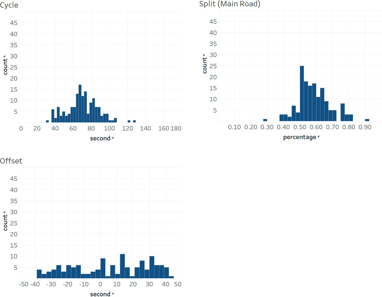
Table 4 shows the results for delay times and CO2 emissions. Each table cell shows the mean value over 50 trials in the first row and the standard deviation in the second row (e.g., ±10.0). In pattern P1, time-only-constrained RL significantly reduced delay times and CO2 emissions compared with the fixed-time control. Coordination-and-time dual-constrained RL showed no significant differences in delay times but significantly decreased CO2 emissions. In pattern P2, RL, unless coordination-only-constrained, significantly decreased delay times and CO2 emissions compared with the fixed-time control. For pattern P3, time-only-constrained RL and dual-constrained RL both significantly decreased delay times and CO2 emissions. In all three patterns, coordination-only-constrained RL significantly increased delay times and CO2 emissions. The significance test used was the Wilcoxon signed-rank test.
| Pattern | Performance index | Fixed-time control | Unconstrained RL | Coordination-only-constrained RL (our method) |
Time-only-constrained RL (our method) |
C/T Dual-constrained RL (our method) |
|---|---|---|---|---|---|---|
| P1 | Delay time + departure wait time | 115.9 (±23.2) |
129.3 (±21.2) |
322.88 (±56.0) |
94.8*** (±12.5) |
113.3 (±16.2) |
| CO2 emissions | 530.3 (±47.5) |
511.1* (±15.1) |
679.7 (±51.5) |
434.8*** (±13.3) |
457.6*** (±12.4) |
|
| P2 | Delay time + departure wait time | 224.3 (±22.0) |
186.8*** (±21.9) |
518.3 (±70.5) |
141.4*** (±17.2) |
174.5*** (±24.0) |
| CO2 emissions | 667.7 (±17.3) |
575.2*** (±23.1) |
750.0 (±28.5) |
492.6*** (±19.1) |
535.2*** (±25.6) |
|
| P3 | Delay time + departure wait time | 97.5 (±12.2) |
99.1 (±11.7) |
182.3 (±35.9) |
77.2*** (±5.5) |
88.9** (±10.1) |
| CO2 emissions | 476.0 (±26.3) |
480.1 (±13.5) |
547.3 (±29.4) |
403.7*** (±9.1) |
425.4*** (±14.2) |
4.3 Discussion
First, the results above revealed a strong correlation between CO2 emissions and delay times. In our experiment, the distance traveled by each vehicle remained unchanged regardless of the signal control type. Hence, CO2 emissions depended on idling time and the number of stops. Reduced idling time and fewer stops naturally entailed lower delay times, resulting in a strong correlation between CO2 emissions and delay times.
Second, with unconstrained RL, the cycle length, splits, and offsets varied significantly as shown in Fig. 3. In particular, an extremely short cycle length of 30 seconds was insufficient to handle the traffic volumes in our experiment. An excessive focus on pursuing individual optimization on the spot probably led to the failure to capture the long-term flow or overall optimum. Moreover, in the real world, human drivers internalize typical signal timings and adjust their intersection behavior accordingly. However, the experimental results show that the signal cycle length and splits varied significantly each time, posing a potential risk of confusion or reduced efficiency. A control system with such highly variable cycle lengths or splits is unsuitable for human drivers and is far from practical at this stage.
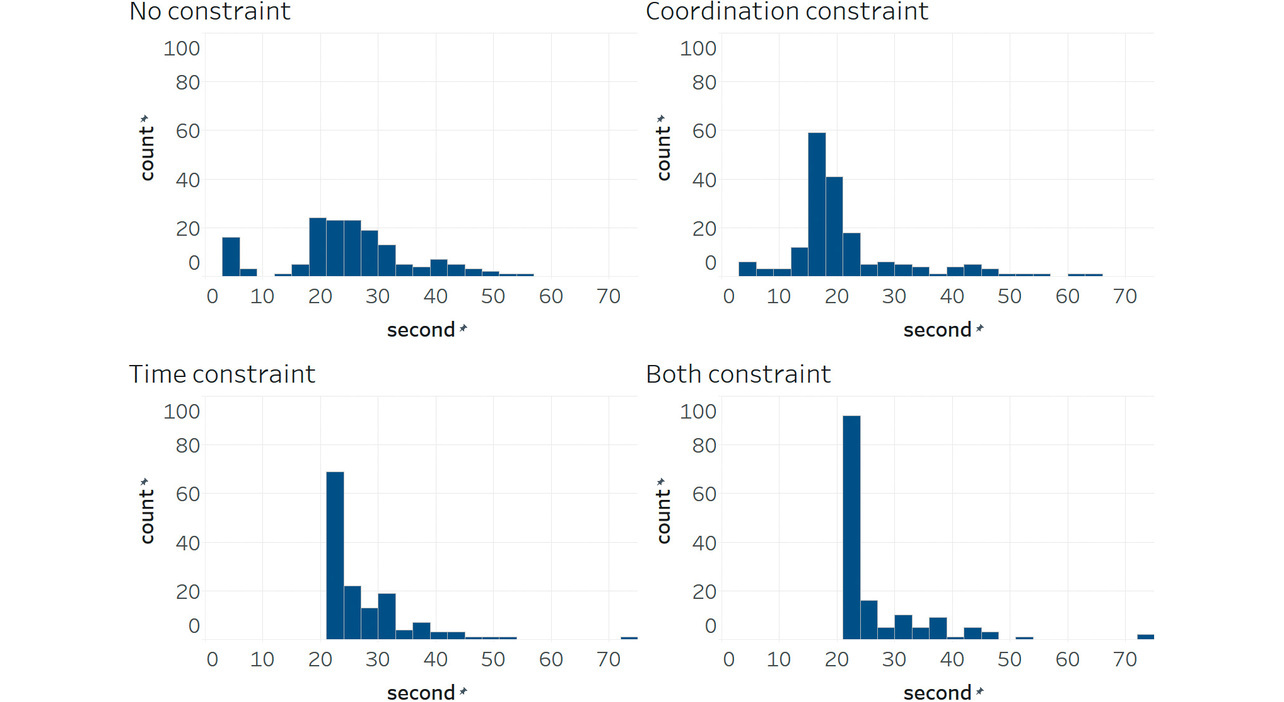
Moreover, Table 4 shows the comparison results between the fixed-time control and constrained RL, revealing that time-only-constrained RL reduced delay times the most. This improvement stemmed from the minimum-seconds constraint, which prevented premature RL-induced phase changes. Fig. 4 shows, as a histogram, the number of seconds for the central-intersection major-road green phase. Fig. 4 suggests that major-road green phases at the heaviest traffic intersection often last only about 3 seconds whether RL is unconstrained or coordination-only-constrained. This phenomenon often causes traffic congestion. On the other hand, with time-constrained RL, major-road green phases lasted at least 21 seconds to allow some traffic flow, which was sufficient to prevent RL-induced misjudgments.
On the other hand, the coordination constraints had no effect in reducing delay times or worsening them. Figs. 5, 6, and 7 show, as histograms, the distributions of the right-intersection cycle length, right-intersection major-road green splits, and offsets between the central and right intersections, respectively. With time-only-constrained RL, the cycle-length distribution converged to a range of 70 to 80 seconds. Meanwhile, splits converged around 60% in distribution. The figures confirm that time-constrained RL properly adjusted the phase time to the flow rate while keeping the cycle length and splits constant. However, offsets were not constant but highly variable.
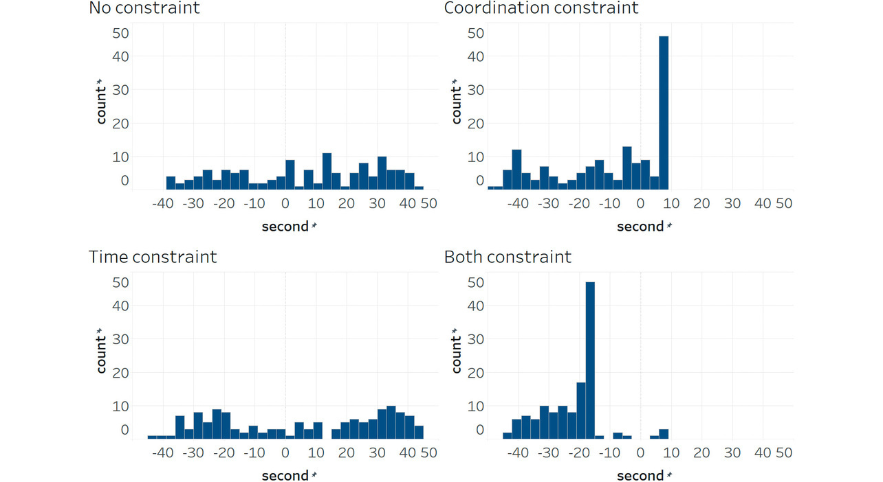
On the other hand, with coordination-constrained RL, offsets converged to some degree, albeit that the cycle length or splits varied considerably. This problem is attributable to poor coordination between the central and right intersections. For example, a green phase continued at the right intersection even though no vehicle remained there just so the central intersection’s phase could catch up. As a result, the cycle length increased, causing traffic congestion. Conversely, an attempt to catch up with the central intersection’s phase would result in a shorter right-intersection cycle length, forcing a phase change in a short time. In particular, the minor roads frequently experienced green truncation after 3 seconds. As a result, queue lengths increased on minor roads, leading to traffic congestion. Forceful application of offset coordination led to highly variable cycle lengths or splits, suggesting an overall increase in delay times or CO2 emissions.
Additionally, for patterns P2 and P3 with higher/lower flow rates than in P1, time-constrained RL led to smaller increases and larger decreases in delay times than fixed-time control. The probable cause was that RL responded to abrupt increases/decreases in the flow rate by adjusting phase times in real time. Presumably, green extension/truncation was used to reduce the number of queued vehicles or to shorten delay times when none existed.
5. Conclusions
In this study, we first showed that conventional RL-based sub-area signal control is impractical because of the large variations in cycle length or split durations. Then, by fusing RL and traffic engineering, we derived and applied phase-time constraints in seconds for RL-based signal control. The resulting stable cycle length and splits demonstrated the effectiveness of our method. However, with the offset type fixed to simultaneous, the constraints intended for signal coordination proved ineffective. If anything, these constraints worsened the results. As for cycle lengths and splits, our time-constrained RL-based signal control method is deemed adequate. On the other hand, with regard to offsets, this constrained RL-based method does not align with findings in traffic engineering. As such, it cannot be called adequate, suggesting that a proper state-action-reward design has yet to be identified. For optimal phase control using RL with well-constrained offsets, we leave it to future studies.
This study demonstrated the potential of an effective signal control method achievable through the fusion of traffic engineering and RL. Such a method would help alleviate traffic congestion, reduce environmental loads, and contribute significantly to future advances in road transportation systems.
Last but not least, we would like to express our gratitude to Mr. Ryuji Ohtani and Mr. Hiroshi Taniguchi of the Business Development Department, Transport Solution Business Headquarters, OMRON Social Solutions Co., Ltd., for their advice on traffic engineering and to Mr. Shota Kanamori of Technology Creation Center, Business Development Administration Headquarters, OMRON Social Solutions Co., Ltd., for his advice during the preparation of this paper.
References
- 1)
- Road Bureau, Ministry of Land, Infrastructure and Transport. “WISENET2050.” (in Japanese), Ministry of Land, Infrastructure and Transport. https://www.mlit.go.jp/policy/shingikai/content/001758738.pdf (Accessed: Mar. 26, 2025).
- 2)
- National Police Agency. “On The Fifth Priority Plan for Social Infrastructure Development (Police-Related Parts).” (in Japanese), National Police Agency. https://www.npa.go.jp/bureau/traffic/seibi2/annzen-shisetu/institut/plan/pdf/juutenkeikaku.pdf (Accessed: Mar. 26, 2025).
- 3)
- M. Izawa and Y. Yamamoto, “Experiments and Considerations on Signal Control Using Deep Reinforcement Learning at Multiple Traffic Flow,” (in Japanese), in Ann. Conf. Japanese Soc. Artif. Intell., 2023, Session ID 3Xin4-69.
- 4)
- K.-L. A. Yau et al., “A survey on reinforcement learning models and algorithms for traffic signal control,” ACM Comput. Surv., vol. 50, no. 3, pp. 1-38, 2017.
- 5)
- F. Rasheed et al., “Deep reinforcement learning for traffic signal control: A review,” IEEE Access, vol. 8, pp. 208016-208044, 2020.
- 6)
- General Corporate Judicial Person Japan Society of Traffic Engineers, Planning and Design of At-Grade Intersections: Basic Edition - Guidelines for Planning, Design, and Traffic Signal Control -, (in Japanese), Maruzen Publishing, 2018, pp. 184-215.
- 7)
- V. Mnih et al., “Human-level control through deep reinforcement learning,” Nature, vol. 518, pp. 529-533, 2015.
- 8)
- M. Wiering, “Multi-agent reinforcement learning for traffic light control,” in ICML ’00: Proc. Seventeenth Int. Conf. Mach. Learn., 2000, pp. 1151-1158.
- 9)
- B. Abdulhai et al., “Reinforcement learning for true adaptive traffic signal control,” J. Transp. Eng., vol. 129, no. 3, pp. 278-285, 2003.
- 10)
- L. Li et al., “Traffic signal timing via deep reinforcement learning,” IEEE/CAA J. Autom. Sin., vol. 3, no. 3, pp. 247-254, 2016.
- 11)
- K. Sato et al., “Development of Traffic Control System by use of Deep Q-Network,” (in Japanese), in Year 2017 Ann. Conf. Japanese Soc. Artif. Intell. (31st), 2017, Session ID 3I2-OS-13b-4.
- 12)
- T. Han et al., “A Study on Possibility of Predictive Deep Reinforcement Learners for Isolated Intersection Signal Control,” (in Japanese), Prod. Res., vol. 73, no. 2, pp. 107-112, 2021.
- 13)
- M. Kuwahara et al., “A Fundamental Study on Signal Parameter Optimization by Reinforcement Learning,” (in Japanese), in 42nd JSTE Conf., 2022, pp. 563-570.
- 14)
- H. Wei et al., “CoLight: Learning network-level cooperation for traffic signal control,” in CIKM ’19: Proc. 28th ACM Int. Conf. Inf. Knowl. Manag., 2019, pp. 1913-1922.
- 15)
- T. Nishi et al., “Traffic signal control based on reinforcement learning with graph convolutional neural nets,” in 21st Int. Conf. Intell. Transp. Syst. (ITSC), 2018, pp. 877-883.
- 16)
- Y. Wang et al., “STMARL: A spatio-temporal multi-agent reinforcement learning approach for cooperative traffic light control,” IEEE Trans. Mobile Comput., vol. 21, no. 6, pp. 2228-2242, 2022.
- 17)
- P. A. Lopez et al., “Microscopic traffic simulation using SUMO,” in 21st Int. Conf. Intell. Transp. Syst. (ITSC), 2018, pp. 2575-2582.
- 18)
- L. N. Alegre, “SUMO-RL.” GitHub. https://github.com/LucasAlegre/sumo-rl (Accessed: Mar. 26, 2025).
The names of products in the text may be trademarks of each company.