


Feasibility Study for Embedded AI Using TensorFlow Lite for Microcontrollers
- Embedded device
- AI Technology
In recent years, deep learning algorithms have been applied to sensing and are contributing to the enhancement of high-precision devices, such as image sensors. This study aims to apply deep learning algorithms to simple sensors that handle one-dimensional signals with the goal of improving accuracy. Because of cost constraints to realize lower product prices, it is challenging to implement large-scale algorithms into simple sensors; however, we aim to achieve this by utilizing embedded deep learning platforms and applying model optimization techniques. In this paper, we use a blood pressure monitor as a practical example of a simple sensor. First, we chose a deep learning platform, and then we described the method for integrating a pretrained model into the blood pressure monitor as well as the techniques for model optimization. Finally, we evaluated the ROM and RAM volumes, accuracy, and execution time, demonstrating the feasibility of the proposed method.
1. Introduction
In recent years, deep learning technology has found applications in sensing algorithms. Deep learning offers the advantages of enhanced accuracy and robustness against noise. The use of deep learning enables high-precision recognition with automatic extraction of complex data patterns. It also enables adaptation to noise-ridden environments and diverse data, allowing for recognition that is free from noise distraction. Deep learning sensing has found applications for a variety of purposes, such as image recognition for autonomous driving vehicles and voice recognition for smart speakers.
OMRON emphasizes sensing as one of its core technologies and has developed a diverse range of sensor products. Besides image sensors and other complex products that handle large-capacity signals, many simple sensor products handle simple one-dimensional signals. Simple sensor products cannot have a high price tag. This cost constraint places limits on the hardware, making it challenging to implement large-scale algorithms, such as those used in deep learning, on these products.
On the other hand, simple sensor products are also always expected to provide more accurate recognition and higher noise adaptation. Therefore, we conducted a feasibility study to further improve sensing accuracy at low cost by integrating deep learning into sensors that handle simple one-dimensional signals.
Deep learning consists of two phases: training and inference. Generally, a training function is based on a more complex algorithm than an inference function and requires high memory capacity and computational complexity. Considering the severity of hardware constraints, we initiated the feasibility study by installing only the inference function on the sensor.
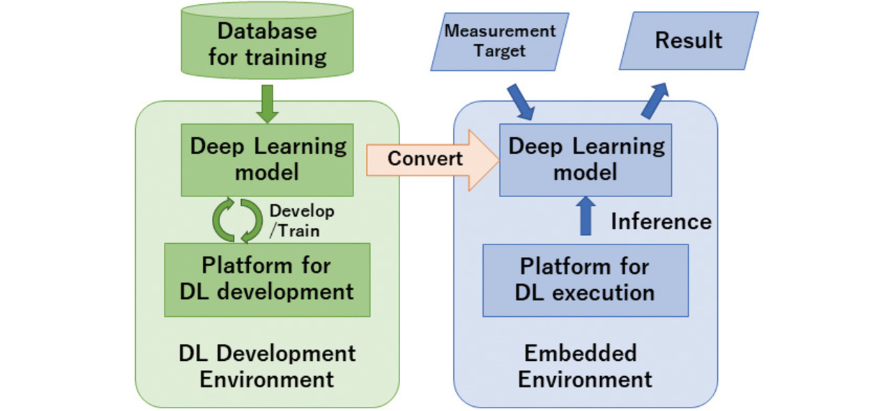
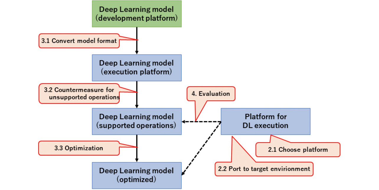
Accordingly, our feasibility study proceeded as follows: developing and training a deep learning model in the algorithm development environment, then installing the model in the sensor, and running it to perform measurement and inference. Fig. 1 shows the structure of the deep learning sensing development explored herein.
The rest of this paper proceeds as follows: Section 2 describes the deep learning development and execution platforms available and then outlines the selections made. Section 3 explains the method of converting the deep learning model developed in the development environment for use in the sensor-embedded environment, followed by the method of compressing the model. Section 4 presents an example of implementation into a blood pressure monitor (sphygmomanometer), along with the results achieved for such parameters as hardware resource usage, runtime, and accuracy to evaluate our proposed method. Fig. 2 shows the flow of these steps. The numbers such as “2.1” found in the balloons in Fig. 2 correspond to the section and subsection numbers in this paper.
2. Platform
Deep learning algorithm development starts with the selection of a deep learning platform and then proceeds to describe and train a model so that it can run on that platform. Running the developed model in an embedded environment requires another platform compatible with the embedded environment.
2.1 Deep learning development platform
Table 1 explains actual examples of platforms for developing deep learning algorithms:
| Platform name | Features |
|---|---|
| PyTorch | An open-source library developed by Facebook. One of the representative deep learning development platforms. Characterized to allow intuitive modeling and widely used in academic research. |
| TensorFlow (Keras) | An open-source library developed by Google. One of the representative deep learning development platforms. There is also a platform called Keras, which is a TensorFlow variant equipped with a high-level API. Numerous peripheral tools are available for model deployment, management, and other purposes. |
| TensorFlow Lite (hereinafter TFLite for short) | A light version of TensorFlow. Optimized for mobile edge devices. TFLite supports a subset of TensorFlow operations. Renamed LiteRT in Sept. 2024. |
| TVM | An open-source deep learning platform developed by Apache. TVM can generate codes optimized for different hardware platforms. |
We adopted PyTorch, valuing its convenience in model building and training.
2.2 Embedded environment platform
We investigated and selected platforms available for running deep learning algorithm models in embedded environments. Our objective was to integrate deep learning into a simple sensor. Considering that the target of our intended implementation example was a blood pressure monitor, we used the following two selection criteria:
- Simple sensors are tightly cost-constrained design-wise and, as hardware, should be selectable with less strict constraints.
- The platform should work OK even with a small-scale microcontroller that cannot be installed with a high-functionality OS, such as Linux.
Table 2 shows the results of investigating platforms for the above criteria:
| Platform name | Features |
|---|---|
| TensorFlow Lite for Microcontrollers (hereinafter TFLM for short) | A light open-source library obtained by further compression of TFLite and compressed enough to run even on embedded microcontrollers. TFLM assumes even microcontrollers with an available memory size of several kilobytes. Its supported operations are a further subset of TFLite operations. It provides a model execution function only, without a model retraining function. |
| microTVM | An open-source library to run TVM models on embedded microcontrollers. microTVM assumes even non-OS installed microcontrollers. It is still under development and likely to undergo major modifications. |
| Edge Impulse | Edge Impulse’s commercial solution. It encompasses a comprehensive range of functions from model development and training to deployment on embedded devices. Its outputs can be generated as C language source code for integration into other software. |
| STM32 X-CUBE-AI |
A free plug-in for STMicro’s microcontroller STM32 series integrated development environment. It imports and converts models developed on other platforms to efficient C language code. It provides a model execution function only. |
Two out of the four platforms, microTVM and TFLM, meet the selection criteria given above. However, the possibility exists that microTVM may undergo major modifications, and the results of our feasibility study may not be fully utilized in future use. Hence, we selected TFLM.
2.3 Target selection
Technical challenges were expected when proceeding directly to implementation into small-scale hardware, the ultimate objective. Therefore, from among microcontroller families that vary in size from small to large, we picked and used those with relatively large-scale hardware to explore implementation. We first achieved successful implementation in large-scale microcontrollers and then considered compression for installation in small-scale microcontrollers to simplify our feasibility study.
From among the STM32 family, which features a wide range of variations, we selected the STM32F769I-DISCO evaluation board. This board is equipped with a comparatively high-level microcontroller, ranked high in those available in the STM32 family. Provided with an external flash memory and an SDRAM, in addition to the microcontroller’s internal memory, it can be expected to work even before being optimized for the embedded environment. Table 3 shows the detailed specifications for the selected target:
| Item | Specification | |
|---|---|---|
| Board name | STM32F769I-DISCO | |
| Microcontroller | STM32F769NIH6 | |
| CPU core | Arm Cortex-M7, 216 MHz | |
| Internal Flash memory | 2 MB | Total ROM size 66 MB |
| External Flash memory | 64 MB | |
| Internal RAM | 512 kB | Total RAM size 16.5 MB |
| External SDRAM | 16 MB | |
2.4 Porting execution
As mentioned above, we adopted TFLM. However, TFLM is distributed in source code form and must be compiled and built to suit the user’s environment. For our feasibility study, we rebuilt the TFLM code into a static library for Cortex-M7 and used it with static linkage to the application. Fig. 3 shows the software configuration for using the TFLM library.
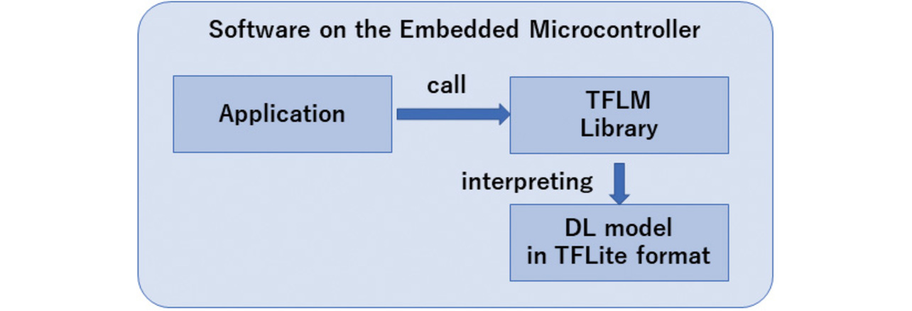
The TFLM library functions as an interpreter of models in TFLite format, translating model descriptions consecutively to perform computations layer by layer.
3. Models
Multiple expression formats exist for deep learning algorithm models. A single platform often supports multiple model formats. Moreover, tools exist for the interconversion of model formats.
3.1 Selection of the model format and conversion tool for use
The deep learning model we used was developed on PyTorch. Running this model on TFLM required converting the model format to a compatible one.
3.1.1 Model formats
Table 4 lists representative deep learning model formats:
| Platform name | Features |
|---|---|
| PyTorch Saved Model | Information of the model developed on PyTorch. While the format and weight information of each layer are stored, interlayer connections are written to the Python program side and, hence, are usable only on PyTorch. |
| ONNX | Abbreviation for Open Neural Network eXchange. An open format usable on various platforms. Both model structure and weight information are stored. |
| TensorFlow | Information of the model developed on TensorFlow. As with ONNX, both model structure and weight information are stored. |
| TFLite | This format has TensorFlow model information replaced with TFLite operations and compressed in size through Flatbuffers (a Google-developed serialization library). |
Table 5 shows the correspondence between the above model formats and the platforms presented in 2.1 and 2.2:
| Model format \ Platform |
PyTorch Saved Model |
ONNX | TensorFlow | TFLite |
|---|---|---|---|---|
| PyTorch | ✓ | ✓ | ||
| TensorFlow | ✓ | |||
| TFLite, TFLM | ✓ | |||
| TVM | ✓ | ✓ | ||
| Edge Impulse | ✓ | ✓ | ✓ | |
| STM32 X-CUBE-AI | ✓ | ✓ |
3.1.2 Conversion tool selection
Multiple model format conversion tools are available for converting deep learning models currently in use. Table 6 shows the interconvertibility and conversion tools for the four model formats above:
| Conversion destination format \ Conversion source format |
PyTorch Saved Model | ONNX | TensorFlow | TFLite |
|---|---|---|---|---|
| PyTorch Saved Model | \ | (1) | ||
| ONNX | (1) | \ | (2) (4) |
(2) |
| TensorFlow | \ | (3) | ||
| TFLite | \ |
Our purpose right here was to convert the deep learning model developed on PyTorch to TFLite format. In this case, either of the following two candidate paths was the option to take:
- A) (1) → (2): The model is exported in ONNX format from PyTorch to onnx2tf for conversion to TFLite format.
- B) (1) → (4) → (3): The model is exported in ONNX format from PyTorch for conversion by onnx-tensorflow to TensorFlow format and then by TensorFlow Lite Converter to TFLite format.
Of the two options, onnx-tensorflow used in path B was last updated in November 2022. As of the time of drafting this paper (November 2024), there had been no update for almost two years. In other words, path B had the drawback of being inaccessible to the latest functions of ONNX and TensorFlow.
Therefore, we selected path A for model conversion. However, onnx2tf does not support all ONNX operations. Suppose that an operation unsupported by onnx2tf is used in an ONNX model. In that case, an error will occur, resulting in a conversion failure that requires some fixes, the details of which are provided immediately below in Subsection 3.2.
3.2 Fixes for unsupported operations
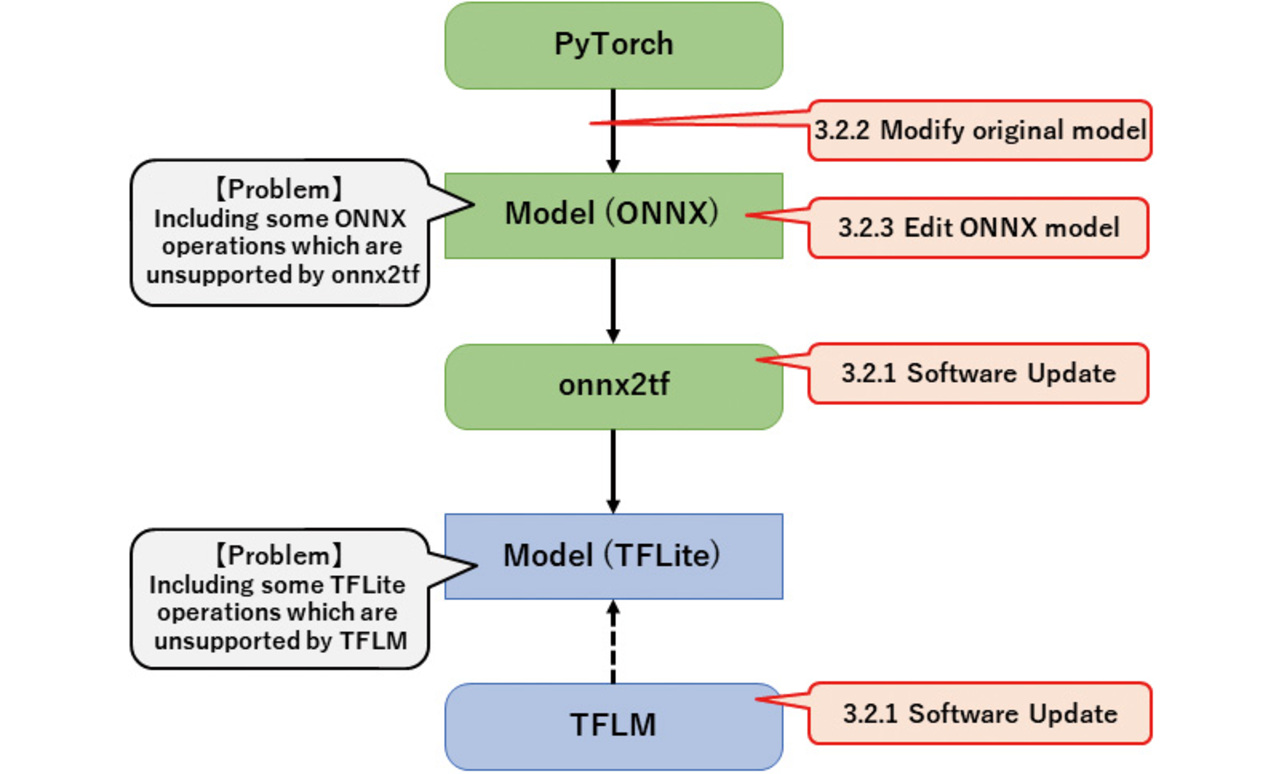
As mentioned in Sub-subsection 3.1.2, some ONNX operations are unsupported by onnx2tf and may not be converted to TFLite format.
Besides, even after successful conversion to TFLite format, another challenge awaits: TFLM does not support all TFLite operations. If any operation unsupported by TFLM is included in the converted TFLite model, an error will occur during program execution.
Fig. 4 outlines these problems and their possible fixes, followed by detailed descriptions. The numbers, such as “3.2.1,” found in the balloons in Fig. 4 correspond to the sub-subsection numbers in this paper.
3.2.1 Software updating
Both onnx2tf and TFLM are open-source software that is under active and continuous development. Operations unsupported by some versions may become executable or be conveted to other simple operations several months later. Regular reference should be made to software update information to check for any change in the status. If a software update can fix the model conversion or execution issue, it is the best solution.
3.2.2 Modifying operations used in the original model
Suppose that an operation unsupported in a converted model format is used in the original model. The required improvement is to modify this operation into one that is supported in the converted model format.
This sub-subsection presents an example of replacing the SELU activation function with the ReLU activation function in a neural network. The ReLU (Rectified Linear Unit) activation function is commonly used in the intermediate layers of deep learning. SELU (Scaled Exponential Linear Unit) was devised as an alternative to ReLU to improve the accuracy of deep learning. Our target algorithm was also developed using SELU. Fig. 5 shows the input and output of each activation function:
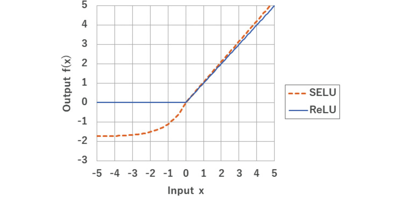
As shown in Fig. 5, the SELU and ReLU outputs significantly differ only when the input x is negative. Because of this difference, a deep learning model may show slightly higher accuracy with the SELU activation function than otherwise4).
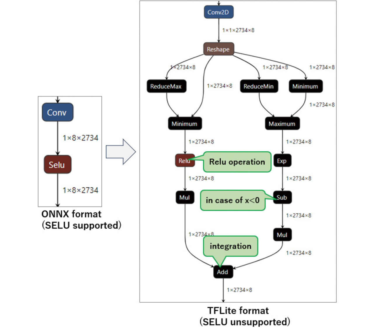
However, TFLite has no SELU-equivalent operations. Hence, when converting an ONNX model that uses a SELU operation, onnx2tf combines multiple operations to generate a model comparable in computation to SELU (See Fig. 6). The model produces calculation results equivalent to those of SELU, albeit with significantly longer computation time and higher memory usage.
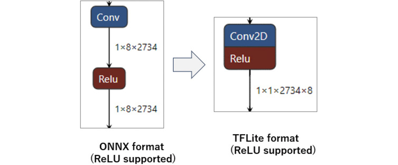
Our solution is to modify the algorithm to use the ReLU activation function compatible with TFLite rather than the SELU activation function during its development on PyTorch. This approach may slightly reduce the accuracy of the deep learning algorithm. However, even after conversion to TFLite format via ONNX format, ReLU operations remain unchanged, significantly saving both computation time and memory usage (see Fig. 7).
3.2.3 ONNX model editing
In some cases, PyTorch generates an ONNX format model containing operations that cannot be converted because they are unsupported by onnx2tf. Even worse, this problem cannot be solved by modifying the PyTorch model.
Conversion with onnx2tf can be achieved by replacing such unsupported operations with other operationally compatible ONNX operations supported by onnx2tf.
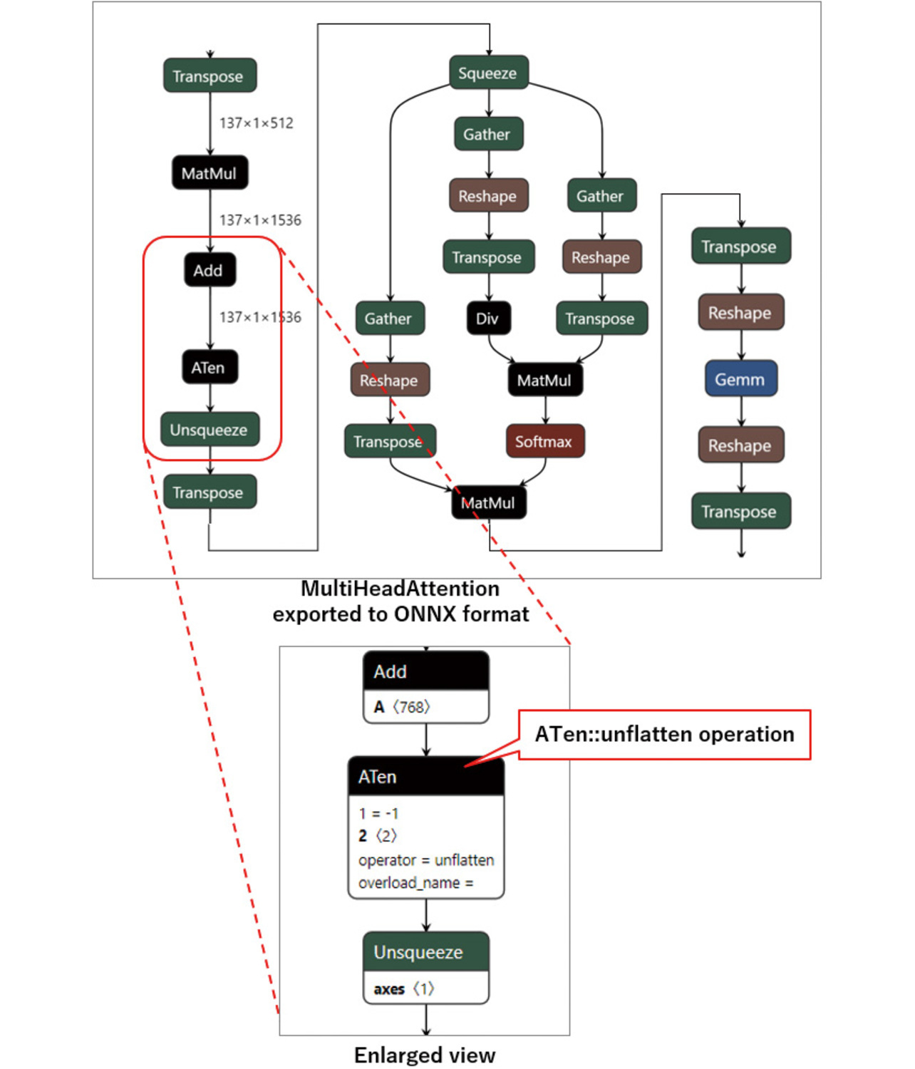
For an illustrative example, Fig. 8 shows a model of the leading part of PyTorch’s MultiHeadAttention operation exported into the ONNX format. ONNX does not support the MultiHeadAttention operation. Hence, a model consisting of a combination of many operations is generated as the output. However, because the ATen::unflatten operation used therein is unsupported by onnx2tf, the output cannot be converted to TFLite format.
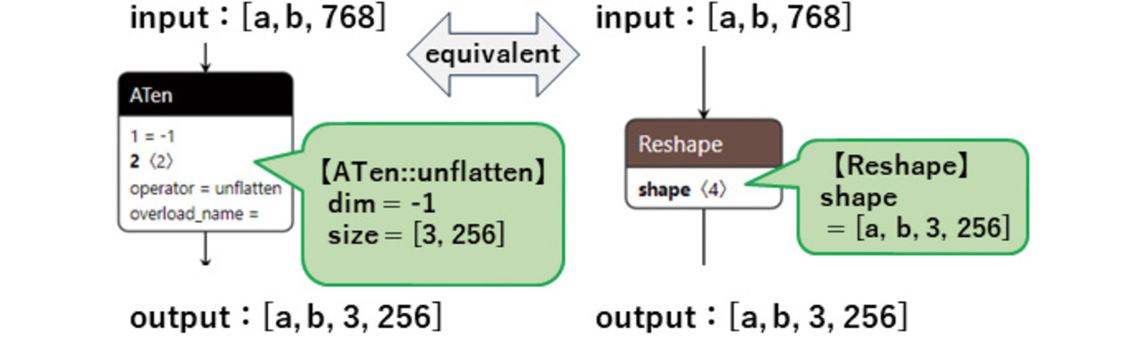
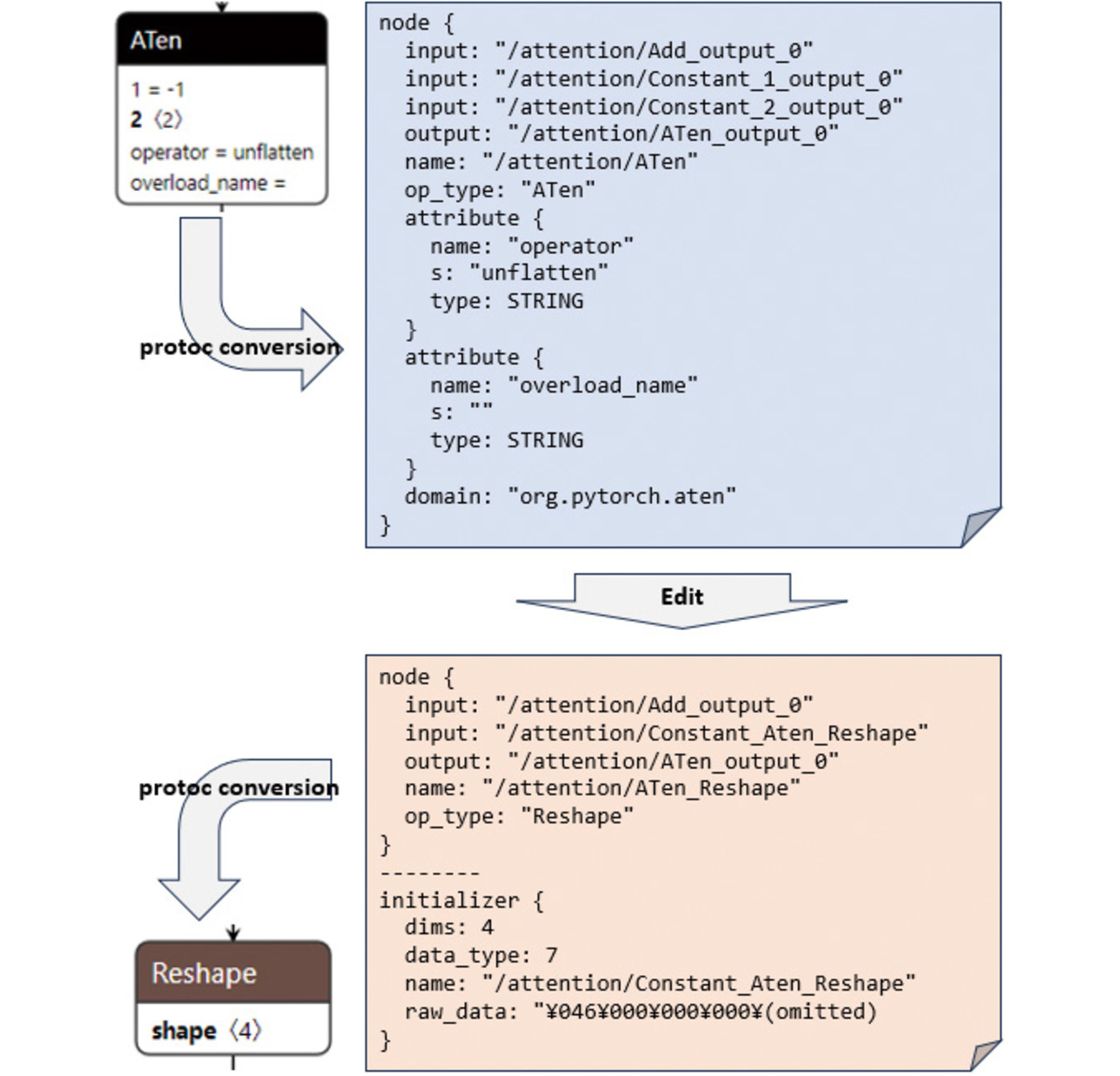
The ATen::unflatten operation converts one dimension specified by “dim” for a multi-dimensional array into a dimension and size specified by “size.” An equivalent operation can be achieved using the Reshape operation, which is a standard feature of ONNX and TFLite. Therefore, the ATen::unflatten operation can be converted functionally intact by replacing it with the Reshape operation through onnx2tf as shown in Fig. 9.
To edit the ONNX model, we used a program called Protocol Buffer Compiler5) (hereinafter “protoc”). Using protoc, we first converted the ONNX model into a text file. Then, we rewrote the operations in the text file and reconverted it back into an ONNX model using protoc again. Fig. 10 shows this procedure:
3.3 Compression
The steps in Subsections 3.1 and 3.2 enabled us to complete a model suitable for the embedded environment. However, the model as built might fail to work due to the limited ROM and RAM volumes available in the embedded environment.
A ROM volume is an area with values fixed during a program run. This area stores program codes and model data. Model data, in particular, and especially the weight data of each neuron of a neural network, occupies most of the ROM volume available. For example, a linear or fully connected layer requires a weight data volume equal to the number of input nodes times the number of output nodes.
On the other hand, a RAM volume is an area used for intermediate computation during a program run. For instance, when a convolution operation is performed, it is necessary to retain data equal to the number of input data×the filter size×the number of channels as intermediate calculation data on the RAM. These data are batch-processed for each neural network layer. It then follows that a model with higher computational complexity per layer requires a larger amount of RAM.
When these required ROM and RAM amounts exceed the ROM and RAM capacities available in the embedded environment, the model needs to be compressed. Sub-subsection 3.3.1 presents the method of performing this compression.
3.3.1 Hyperparameter tuning
A parameter that specifies the size or the like of each layer in a model is called a hyperparameter. The tuning of hyperparameters plays a crucial role in the development of a deep learning algorithm. The size of the model varies depending on the hyperparameter settings. So does its accuracy. Increasing the size of the model does not necessarily improve its accuracy. A balanced combination of size and accuracy must be explored.
This tuning of a hyperparameter must be performed in the deep learning algorithm development environment. An automatic search tool, Optuna6), is used to repeat retraining and evaluation, changing the candidate combination of parameters to search for a combination for higher accuracy.
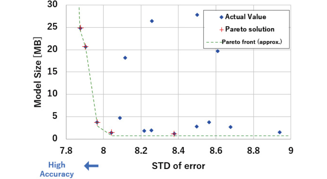
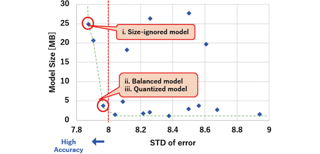
For example, let us run a search with approximately three to five options assigned to each of the ten hyperparameters in a deep learning algorithm. The search results yield multiple instances of the same solution that say, “No result available for a combination that makes a model smaller in size and higher in accuracy.” When tuning is viewed as an optimization problem between model size and accuracy, these solutions are referred to as Pareto solutions. Fig. 11 shows the measured values and Pareto solutions. From among the Pareto solutions, select tuning results that meet the model size and accuracy requirements.
For the tuning results thus obtained, the steps in Subsections 3.1 and 3.2 are repeated to obtain a model installable in the embedded environment.
3.3.2 Model quantization
One of the general methods for compressing deep learning models is the quantization of weight data. The term quantization refers to achieving reduced computational complexity and memory usage by turning floating-point numbers into fixed-point numbers and expressing them as low-bit-count integer types.
The quantization operation for a deep learning model is performed by specifying the options for model conversion, as outlined in Subsection 3.1. When an input data constellation is given, the numerical value range for each layer of the neural network is automatically calculated, thereby assigning an operation to contain data within that range and convert them into integers. Fig. 12 shows a conceptual diagram:
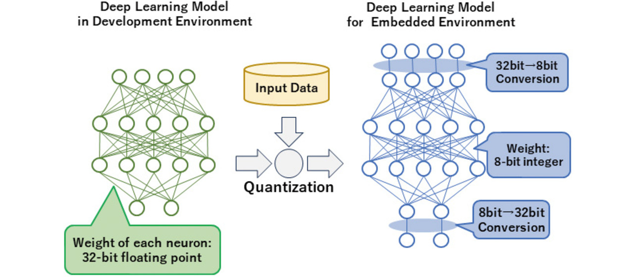
When quantized from 32-bit to 8-bit, the model is compressed to approximately 1/4 of its original size. On the one hand, this method does not affect the algorithm. On the other hand, it doesn’t optimize the algorithm for quantization, which poses an accuracy challenge.
4. Evaluation
Section 4 evaluates the pros and cons of the deep learning model embedding methods as presented in Sections 2 and 3 based on the results of applying them to an algorithm and hardware designed for actual sensor products.
4.1 Evaluation targets
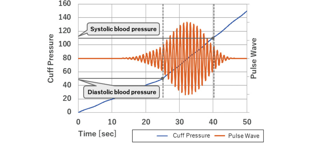
This section uses a blood pressure monitor (sphygmomanometer) as an example of the intended target products. A blood pressure monitor is a sensor that produces two numerical outputs of the maximal or systolic blood pressure (SBP) value and the minimal or diastolic blood pressure (DBP) value from two sets of one-dimensional time-series input data, cuff pressure data obtained by the compression of the blood vessels with an inflated cuff and pulse wave data generated during cardiac contractions. Fig. 13 shows the cuff pressure and pulse wave inputs to a inflation-based blood pressure monitor:
Generally, blood pressure monitor products need to be moderately priced compared with PCs and other electronic devices. As such, they are controlled by a microcontroller with a capacity and speed several orders of magnitude lower than those of PC CPUs. Therefore, they have a hardware constraint, which is the difficulty in installing a deep learning algorithm developed on a PC as is. Table 7 is an excerpted reproduction of the hardware specifications for the implementation target selected in Subsection 2.3:
| Item | Specification | Remarks |
|---|---|---|
| CPU core | Cortex M7 | With built-in FPU |
| Clock frequency | 216 MHz | |
| Flash ROM volume | 66 MB | 2 MB internal and 64 MB external |
| RAM volume | 16.5 MB | 532 kB internal and 16 MB external |
We prepared the following three different evaluation target models:
-
i.
Size-ignored model
A model developed in the algorithm development environment with top priority given to accuracy. Selected as the model with the highest accuracy in the hyperparameter tuning results in Sub-subsection 3.3.1. -
ii.
Size-accuracy balanced model
A model is selected based on the tuning result in Sub-subsection 3.3.1 to strike a balance between size and accuracy. Selected as the model smallest in size in the range within which the standard deviation of error, one of the two evaluation criteria in Subsection 4.2, meets the criterion. -
iii.
Quantized model
A model obtained by quantizing the balanced model above using the method in Sub-subsection 3.3.2.
Fig. 14 shows the correspondence between the models and parameter tuning results above:
4.2 Evaluation criteria
This section evaluates Models i, ii, and iii presented in Subsection 4.1 for the following indicators.
- MAE (mean absolute error)
An indicator of accuracy. Required to be 5 or below according to an international standard for sphygmomanometers7). - SDE (standard deviation of error)
An indicator of accuracy. Required to be 8 or below according to an international standard for sphygmomanometers7). - Runtime
The time required to calculate the blood pressure values from measurement data. A commercially available sphygmomanometer took approximately 3 seconds to show the blood pressure values after completing the measurement. Hence, a runtime of less than 3 seconds is desired. - ROM volume
- RAM volume
4.3 Evaluation method and evaluation results
We entered approximately 500 pairs of pulse wave and cuff pressure data into the deep learning models for testing, allowing them to run estimations and calculate the errors between SBP output and ground truth values. Fig. 15 shows a schematic diagram of this flow:
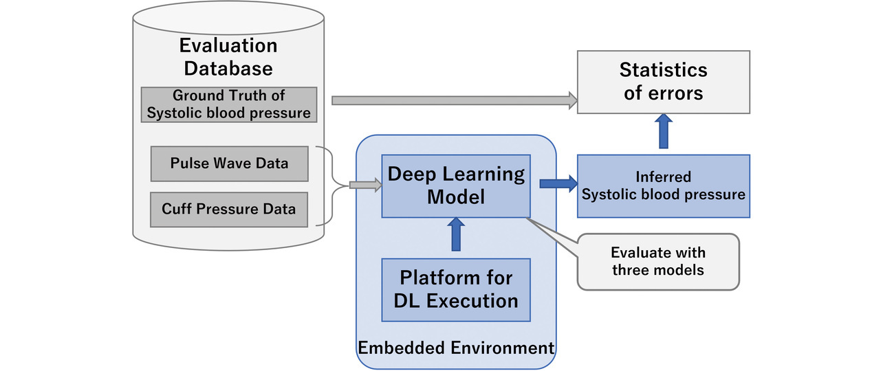
Table 8 shows the evaluation results for the three different evaluation target models:
| Indicator | Hyperparameter tuning model | iii. Quantized model | |
|---|---|---|---|
| i. Size-ignored | ii. Balanced | ||
| Accuracy (MAE) | 6.66 | 6.74 | 8.16 |
| Accuracy (SDE) | 7.83 | 7.97 | 10.71 |
| Runtime [ms] | 12,214 | 1,938 | 348 |
| ROM volume [MB] | 18.37 | 3.72 | 0.98 |
| RAM volume [kB] | 663.4 | 221.0 | 63.7 |
- The size-ignored model was evaluated for accuracy with the algorithm development environment. Though large, the ROM and RAM volumes remained within the limit for mounting on our target, allowing the model to run even on the target. However, its runtime exceeded 12 seconds, making the model too slow for practical use in a sphygmomanometer.
- The size-accuracy balanced model had a ROM volume of over 2 MB. As such, it required external flash ROM. However, with a RAM volume of 221 kB, it was sized to run with microcontroller-integrated RAM alone. Moreover, its runtime was within 2 seconds, shorter than achievable with current commercially available products, making the model acceptably fast.
- The quantized model had a ROM volume of 0.98 MB and a RAM volume of 63.7 kB, both of which fell within the capacities of the microcontroller’s internal memory. A runtime of 348 ms (0.348 seconds) was achieved, enabling the model to run at a practical speed. This model exhibited a significant deterioration in accuracy, failing to meet the SDE of less than 8 as specified in the international standard for sphygmomanometers.
- None of these models met the MAE of less than 5, the mean absolute error indicator. However, our objective was not to achieve improved accuracy from the existing technology but to demonstrate the feasibility of embedding deep learning technology. Hence, despite not meeting this indicator, our objective was still achieved.
Based on the above, we successfully developed a deep learning algorithm that could run in the embedded environment designed for sphygmomanometers. Additionally, we confirmed that quantization could significantly reduce runtime and the volumes of ROM and RAM.
5. Conclusions
5.1 Our achievements so far
This paper presented a procedure established for running our deep learning algorithm in the target embedded environment. We converted a deep learning model developed on PyTorch, a deep learning algorithm development environment, for use on TensorFlow Lite for Microcontrollers, the execution environment for deep learning algorithms for embedded use. To address several challenges resulting from the conversion, we presented specific solutions. Moreover, we presented two methods of hyperparameter tuning and model quantization as the means of model compression to meet the memory and runtime constraints required for the embedded environment. Finally, we ran the compressed model on the microcontroller to demonstrate the feasibility of operating our deep learning algorithm in embedded environments.
The procedure presented in Section 3 can be applied to diverse developments. We conducted an implementation feasibility study, using a sphygmomanometer as an example, to verify that our proposed procedure is moderately feasible. The applicability of our deep learning algorithm may not be limited to sphygmomanometers but may also extend to sensors that perform signal processing on one-dimensional data strings. Examples of likely candidates include sensors that measure physical quantities such as light and temperature.
5.2 Future work
Our hyperparameter tuning enabled accuracy retention to a degree but fell short of keeping errors within the acceptable range for the microcontroller’s internal memory, leaving room for improvement. In our approach, quantization resulted in significantly reduced accuracy. The means of achieving accuracy retention simultaneously with quantization include, for example, a method that develops a model to remain accurate in its quantized state by proceeding with a model in its quantized state from its training phase in the development environment. We continue this study to pursue an optimal balance between size reduction and accuracy toward future practical applications.
References
- 1)
- Katsuya Hyodo. “onnx2tf.” GitHub. https://github.com/PINTO0309/onnx2tf (Accessed: Nov. 1, 2024).
- 2)
- Google. “TensorFlow Lite Converter.” TensorFlow. https://www.tensorflow.org/lite/convert?hl=ja (Accessed: Nov. 1, 2024).
- 3)
- Open Neural Network Exchange. “TensorFlow Backend for ONNX.” GitHub. https://github.com/onnx/onnx-tensorflow (Accessed: Nov. 1, 2024).
- 4)
- Dabal Pedamonti. “Comparison of non-linear activation functions for deep neural networks on MNIST classification task.” arXiv. https://arxiv.org/abs/1804.02763 (Accessed: Apr. 8, 2018).
- 5)
- Google. “Protocol Buffers - Googleʼs data interchange format.”GitHub. https://github.com/protocolbuffers/protobuf (Accessed: Nov. 5, 2024).
- 6)
- T. Akiba et al., “Optuna: A Next-generation Hyperparameter Optimization Framework,” in Proc. ACM SIGKDD Int. Conf. Knowl. Discovery Data Min., 2019, pp. 2623-2631.
- 7)
- Non-invasive sphygmomanometers - Part 2: Clinical investigation of intermittent automated measurement type, ISO 81060-2, 2018.
The names of products in the text may be trademarks of each company.