


Proposal of Concept Drift Detection in Factory Automation (FA) Domain
- Abnormal Detection
- Concept Drift
- Causal Relationship
- Machine Learning
In recent years, with the trend of machine learning, there has been an increase in the application of anomaly detection using machine learning to predict product defects in Factory Automation (FA) domain. However, because of the diversification of products and the efficiency of the manufacturing processes, frequency of the 4M (Man, Machine, Material, Method) changes have increased. If the anomaly detection model, which was operational before the 4M changes, continues to be used, false detections happen. And they can lead to an increase in product defects.
This phenomenon, where the relationship between input data and inference results changes during the operation of anomaly detection from the time of learning, is referred to as concept drift. Previously, concept drift by 4M changes has been measured using such means as averages. However, these methods have been problematic because of delayed detection and issues with real-time performance.
This paper proposes a method that integrates multiple anomaly detection models by considering causal relationships, thereby achieving both the prediction of product defects and the detection of concept drift caused by 4M changes. Furthermore, the effectiveness of the proposed method was verified using an injection molding machine utilized at the manufacturing sites.
1. Introduction
Following the recent spread of machine learning, the factory automation (FA) field has seen increases in the examples of machine learning-based product defect prediction used at manufacturing sites. In many cases, manufacturing sites operate anomaly detection tools suitable for small amounts of defect label data to improve their quality ratios. Omron has also commercialized an AI-equipped machine automation controller1). This product provides anomaly detection using sensing data inputs collected from manufacturing equipment.
However, recent diversified products and complicated manufacturing technologies have led to increasingly more frequent encounters with 4M changes, which refer to changes in the man, machine, material, and method at FA manufacturing sites. Continuously operating an outdated anomaly detection model, even after a 4M change, can result in false detections. A delayed response to this problem leads to a higher product defect rate.
Factors in the 4M changes may cause the relationship between input data and inference results to change during an anomaly detection operation from what it was at the point of pre-operational learning. Such a change is called a concept drift2). Conventional measures to address such a problem include moving average-based methods and the average-run-length (ARL) method, the latter of which evaluates the sequences of highs/lows relative to the center values on control charts3). However, these methods have problems with real-timeliness, operational skills, and workloads.
With causality in mind, we identified a group of variables representing product defect factors and a group of 4M-change variables affecting them. In this paper, we propose a method that integrates multiple anomaly detection models generated from each group of variables. Our proposed method aims to achieve compatibility between product defect sign detection and 4M change-induced concept drift detection. In this paper, we also present the results of a verification experiment performed using an injection molding machine found on manufacturing sites to demonstrate that our proposed method can detect both types of events.
2. Challenge
This section first outlines the behavior of the system of interest. It then explains the challenge posed by concept drifts encountered while detecting anomalies under analysis.
2.1 System of interest
Fig. 1 shows the injection molding machine of interest.
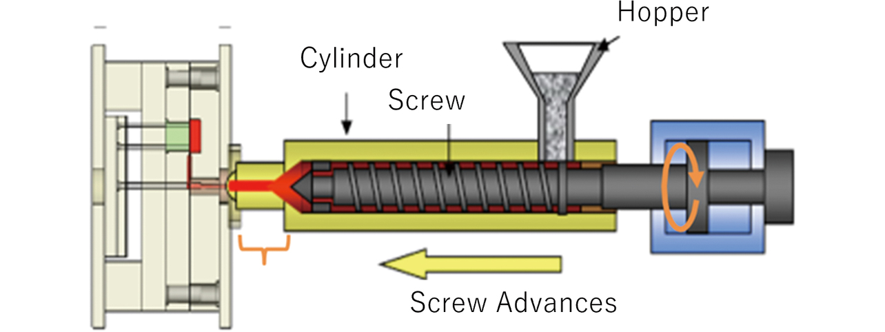
This injection molding machine injects plasticized and molten resin in the mold (highlighted red in Fig. 1) into the pipe (left in Fig. 1) rapidly under high pressure, enabling precision-mass production of plastic parts with complex shapes4). It also characteristically accommodates multi-type production by adjusting the injection condition changes for each product type. However, if it fails to fill sufficient resin into the mold due to improper settings or residual resin on the screw, defective products may result. The variables of pressure, time, and injection rate are monitored to detect any signs of defective products. When any preset threshold is exceeded, corrective measures, such as machine setting adjustment or cleaning, can be implemented before a defect occurs.
2.2 Challenge
Approximately 70 different types of variables exist that represent molding defect factors. These variables include those mentioned in the previous subsection, in other words, pressure, time, and injection rate. The conventional response to defects encountered under specific conditions is to select variables with a high contribution based on decision-tree importance scores and build an anomaly detection model to monitor signs of molding defects5). In the case of anomaly detection, only normal data are necessary to build a learning model. Hence, it is an effective method for manufacturing sites with lesser defect data. This method is adopted for the AI-equipped machine automation controller, one of Omron’s products. Fig. 2 shows an example of anomaly detection performed using a similar conventional method.
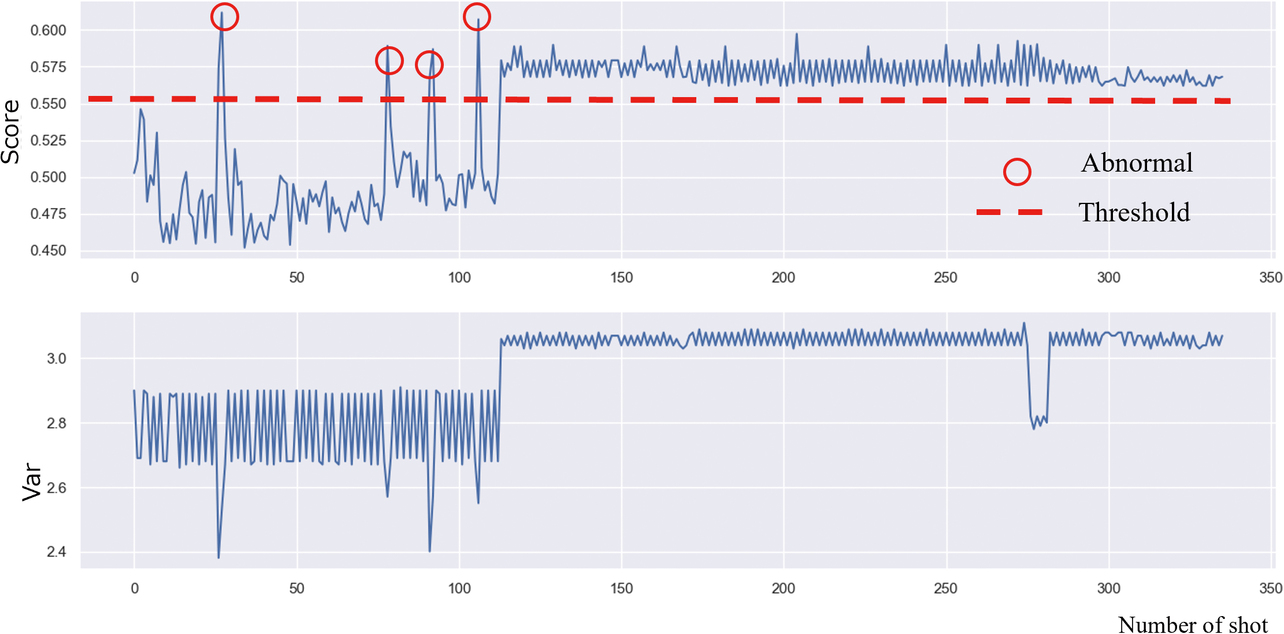
The upper graph in Fig. 2 shows an anomaly score as the anomaly detection index, while the lower graph shows one of the explanatory variables representing the anomaly detection model. Molding defect sign detection was performed with this model set to an anomaly score threshold of 0.555. The left/first half of the upper graph in Fig. 2 shows anomaly detection results obtained as intended. However, the right/second half shows the threshold constantly exceeded for the 114th and subsequent shots. The cause was the change in the product type produced with the 114th and subsequent shots. As a result, anomalies after the type change became impossible to detect correctly. Relearning at the point of the 114th shot was necessary to detect defects after the type change. At this point, however, whether to perform relearning was impossible to determine. Hence, production continued for a long time without detecting defects. Immediate type change detection followed by relearning would reduce product defect rate. Hence, our challenge was to detect type changes while molding defect sign detection was in operation.
2.3 Requirements for our proposed method
The previous section defined concept drift as a change in the input data-inference result relationship between the point of learning and during an anomaly detection operation. Concept drifts fall into those that gradually change over time and those that abruptly change. The latter category includes 4M changes, such as a change in the product type to be manufactured. The molding machine of interest is required to support real-time defect sign detection to prevent defective product production.
Accordingly, the challenge presented in the previous subsection can be solved by a method that detects abrupt concept drifts during anomaly detection operations at a manufacturing site.
The conventional method that most likely comes first to mind is one that detects states with a continuously exceeded threshold. Specifically, the method would be based on moving average or control chart ARL. However, a moving average-based method would be too slow in response to track abrupt changes and, hence, unsuitable in terms of real-timeliness. Meanwhile, an ARL-based method would be challenging skill-wise because its control values and other non-threshold parameters are hard to determine. Accordingly, a desirable method should eliminate the need for parameter adjustment, allowing for skill-free operation.
An alternative idea may be to build an anomaly detection model for each product type. However, most injection molding machines accommodate more than ten types to cope with recent product diversification. Building and operating an anomaly detection model for each type would pose operational workload-related problems, including data management, model generation, and threshold settings. Hence, a desirable solution should include a single anomaly detection model to monitor during operation.
From the above, our proposed solution should first and foremost require concept drift detection with real-timeliness. Additional requirements should include skill-free operation involving no parameter adjustment and compatibility between product defect sign detection and type change detection as 4M changes.
3. Our proposed method
3.1 Outline of our proposed method
We adopted the Isolation Forest algorithm6) from a broad range of anomaly detection algorithms7) for our proposed method. The Isolation Forest features high-speed inferencing and supports real-time detection. Besides, its operation requires no consideration of non-threshold parameters and involves few problems with operational skills. This paper considers using the Isolation Forest to establish compatibility between product defect sign detection and type change detection as 4M changes and integrate them into a unified anomaly detection model. The Isolation Forest only requires setting a threshold for defect sign detection and another for type change detection that enables reduced operational workloads, less demanding skills, and improved real-timeliness.
In what follows, Subsection 3.2 outlines the Isolation Forest, Subsection 3.3 explains the effect and factor identification process, respectively, for product type and defect factors, Subsection 3.4 describes the anomaly detection integration process, and Subsection 3.5 presents our method for anomaly score calculation.
3.2 Outline of the Isolation Forest
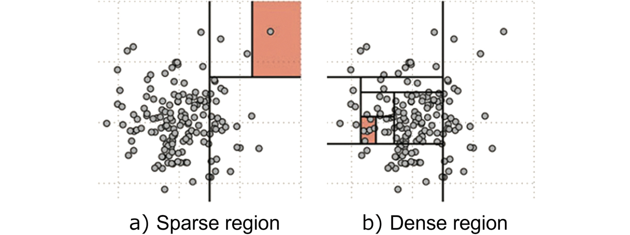
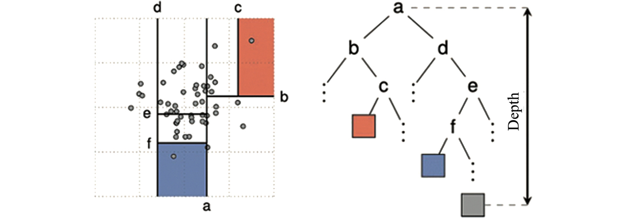
The Isolation Forest is an anomaly detection algorithm that builds a model from unlabeled learning data and classifies data into normal and abnormal data based on data sparsity/density. Whether data are sparse or dense is determined based on the required number of partitions to split the data until each point is isolated. A relatively small number of partitions is required to split the sparse region points until each point is isolated as shown in Fig. 3a). Meanwhile, a larger number of partitions is required to do the same to the dense region points as shown in Fig. 3b). As shown in Fig. 4, the required number of partitions is the depth of a binary tree based on which the anomaly score calculation is performed.
The binary tree is built from the sampled learning dataset X = {x1, x2, x3, ... xn} to calculate the anomaly score by Eq. (1) from the depth information of the data to be evaluated. More specifically, the following operation is performed:
where h(x) represents the depth of the evaluation point x in the binary tree built of n points of sampled data; for example, in a set of 256 (= 28) points of sampled data, the binary tree can have a depth of 1 to 8 E(h(x)), the expected depth value of the evaluation point x in multiple binary trees is normalized, whereby the anomaly score takes a range of (0,1]. A threshold is set for this anomaly score to perform anomaly detection. Incidentally, γ is the Euler’s constant (≈ 0.57721).
3.3 Identification of effects and factors
This subsection describes how variables representing product defects and type change factors are identified.
3.3.1 Identification of product defect factors
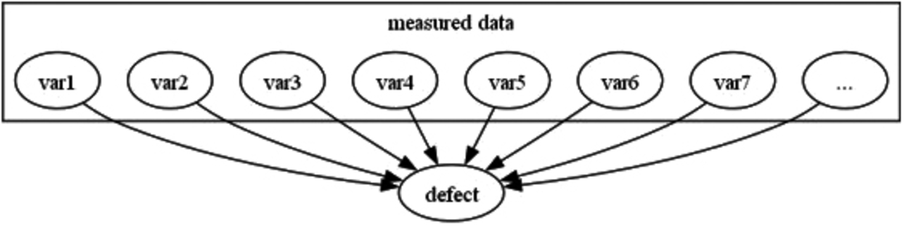
The first things to identify are the factors leading to molding defects. Let a set of variables collected from the molding machine be measured data. Fig. 5 shows how these variables (var1, var2, var3, var4, …) are involved in the occurrence of a molding defect.
A set of variables representing the identified molding defect factors is calculated by Eq. (2) below:
where x is a set of variables, including temperature and pressure collected from the molding machine. Importancedefect-factors calculates the Random Forest importance of x with defective and non-defective products labeled discrete variables. Xdefect-factors is a set of variables conditioned by a user-defined threshold Thdefect-factors for the importance thus calculated.
3.3.2 Identification of the variables affected by a product type change
The next things to identify are the variables affected by a product type change. Fig. 6 shows how a type change affects the variables collected from the molding machine.
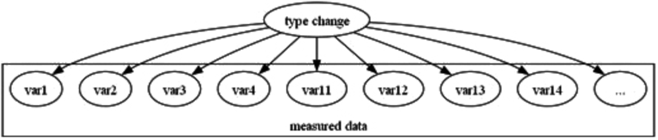
The variables affected by the type change consist of the variables representing the molding defect factors (var1, var2, var3, var4) shown in Fig. 5 and variables not representing molding defect factors (var11, var12, var13, var14, …).
Then, a set of variables affected by the type change is calculated by Eq. (3):
Xtype-factors, the set of variables affected by the type change, is the importance conditioned by a user-defined threshold with respect to x with the type labeled with discrete variables, similarly as in Eq. (2).
3.4 Anomaly detection model generation
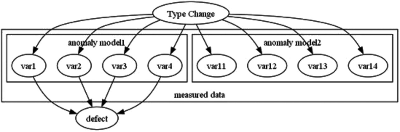
This subsection describes the process of generating anomaly detection models for quality defect sign detection and type change detection. As shown in Fig. 7, the quality defect sign detection model (Anomaly Model 1) consists of a set of variables affected by a type change and representing defect factors. The type change detection model (Anomaly Model 2) consists of a set of variables affected by the type change but not representing defect factors.
3.4.1 Anomaly detection model for product defect signs
Eq. (4) represents the learning data for the anomaly detection model for product defect sign detection:
Thus, Xanomaly-model1 is the Cartesian product of the product defect factors’ and product type’s effects.
Then, Eq. (5) shows the calculation method for our model’s anomaly score, sanomaly-model1:
where xanomaly-model1 is the data evaluated by the anomaly detection model consisting of the learning data Xanomaly-model1.
The first of the two thresholds used in our model is a user-defined Thresholdanomaly-model1 with normal learning data not exceeding the anomaly score.
3.4.2 Anomaly detection model for product type changes
Eq. (6) represents the learning data for the anomaly detection model for product type change detection:
Thus, Xanomaly-model2 is the Cartesian product of a non-product defect factor set and a product type-affected set.
Then, similarly to Eq. (5), Eq. (7) shows the calculation method for our model’s anomaly score, sanomaly-model2:
xanomaly-model2 is the data evaluated by the anomaly detection model consisting of the learning data Xanomaly-model2.
The second of the two thresholds used in our model is a user-defined Thresholdanomaly-model2 with normal learning data not exceeding the anomaly score.
3.5 Anomaly score calculation
This subsection explains the calculation and threshold of the anomaly score that integrates Anomaly Model 1 for molding defect sign detection with Anomaly Model 2 for type change detection.
Eq. (8) represents the anomaly score that integrates the multiple anomaly detection models proposed in our method:
As shown in Subsection 3.2, the Isolation Forest anomaly score is obtained as the normalization of the expected depth value for the data evaluated. Hence, when evaluated by the two anomaly detection models, the same data xunion can be represented as the square root of the multiplication of the anomaly score from the law of exponents.
The integrated anomaly score sunion takes the same range of (0,1] as the Isolation Forest anomaly score. Therefore, Thresholdanomaly-model1, explained in Sub-subsection 3.3.1, is used as the threshold for molding defect sign detection, while Thresholdanomaly-model2 is used as the threshold for type change detection.
4. Verification
This section presents the results of verifying the effectiveness of our proposed method using the data collected from the injection molding machine shown in Subsection 2.1. The conventional method compared was an anomaly detection method using a conventional method similar to the AI-equipped machine automation controller mentioned in Subsection 2.2.
4.1 Details of the verification
Table 1 summarizes the data we verified:
| Product type | Shot count | Number of collected variables | Number of shots to be determined as detected anomalies |
|---|---|---|---|
| A | 113 | 70 | 4 |
| B | 223 | 70 | 70 |
The products manufactured fell into two types. After 113 shots worth of Type A were manufactured, a transition occurred to the manufacturing of Type B. The verification presented herein aimed to detect the changeover to Type B after determining that four shots were detected as defect signs for Type A.
Because of confidentiality, this paper does not present specific details of the explanatory variables.
4.2 Anomaly detection models
Table 2 shows the details of the anomaly detection models generated by our proposed method.
| Anomaly detection model |
Anomaly detection model’s explanatory variables | Sample size |
|---|---|---|
| Anomaly Model 1 | var1, var2, var3, var4 | 40 |
| Anomaly Model 2 | var11, var12, var13, var14 | 40 |
The anomaly detection models generated were the two types presented in Subsection 3.4, Anomaly Models 1 and 2. The sample size for the model generation here was 40 shots worth of Product Type A. Four explanatory variables were selected for each anomaly model according to Subsection 3.3. Fig. 8 shows the histograms for the respective explanatory variables.
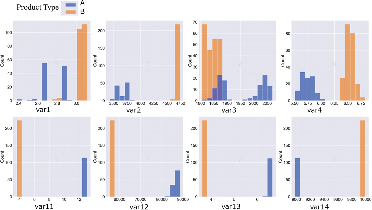
The variables representing Anomaly Model 1, i.e., var1, var2, var3, and var4, showed variations in distribution, especially for Product Type A containing defects. Anomaly detection operations using these variables were performed for product defect sign detection. On the other hand, the variables representing Anomaly Model 2, i.e., var11, var12, var13, and var14, showed no product type-specific variations in distribution. These observations reveal that anomaly detection using these variables is suitable for product type determination.
4.3 Verification results
Per Sub-subsections 3.4.1 and 3.4.2, we set two values not exceeding the normal anomaly scores as Thresholds 1 and 2 for the anomaly detection models, Anomaly Models 1 and 2, respectively, based on the anomaly scores for the learned results. Table 3 shows the thresholds for Anomaly Models 1 and 2, respectively:
| Anomaly detection model |
Threshold’s name |
Threshold’s purpose |
Threshold |
|---|---|---|---|
| Anomaly Model 1 | Threshold 1 | Defect sign detection | 0.550 |
| Anomaly Model 2 | Threshold 2 | Product type change detection | 0.570 |
Fig. 9 shows the results of anomaly score evaluation by our proposed method:
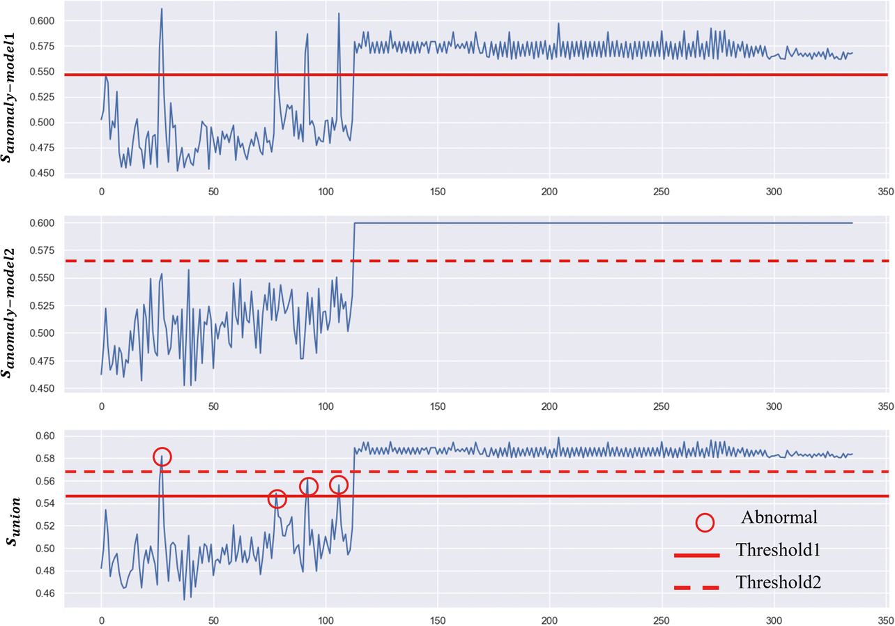
These graphs are arranged from top to bottom for Anomaly Model 1’s anomaly score, sanomaly-model1, Anomaly Model 2’s anomaly score, sanomaly-model2, and the integrated anomaly detection model’s anomaly score sunion.
In the first graph, sanomaly-model1 shows the results for the conventional method, in other words, the anomaly detection model built of variables representing product defect factors. It reveals that while the four defective shots in the first half were correctly determined as such, the post-type change shots were all determined defective with the anomaly score threshold constantly exceeded.
In the second graph, sanomaly-model2 shows that the post-type change shots were all successfully detected, although product defect determination failed.
In the third graph, sunion shows the results of our proposed method. The product defect signs and the post-type change shots were all successfully detected. Moreover, the product defect-vs.-type change differentiation by Thresholds 1 and 2 was successful with the single exception of the 37th shot.
Table 4 summarizes the evaluation results for our verification:
| Product type |
Shot count |
Number of collected variables |
Number of shots to be determined as detected anomalies | Accuracy |
|---|---|---|---|---|
| A | 113 | 70 | 4 (defect sign) | 99.1% |
| B | 223 | 70 | 223 (product type) | 100% |
The evaluation data for Product Type A showed an accuracy of 99.1% due to the unsuccessful product defect-vs.-type change differentiation for the 37th shot data. The evaluation data for Product Type B shows that the post-type change shots were all correctly detected.
4.4 Discussion
The verification data showed an accuracy of 99.1% and 100% in the graph’s Product Type A and B sections, respectively. The anomaly score shown by our proposed method was observed to behave almost as intended, albeit with one shot incorrectly detected.
The 37th shot showed an anomaly score exceeding Threshold 2 and was incorrectly detected as a post-type change shot instead of a pre-type change shot. The cause was probably that the anomaly score variation range differed between the graph’s first and second halves. A check with sanomaly-model2 reveals that the anomaly score varied from 0.45 to 0.55 in the first half/Type A section but remained almost constant in the second half/Type B section. The integration of the sanomaly-model1 and sanomaly-model2, i.e., sunion, was also probably affected by the anomaly score variations in the first half/Type A section, causing the anomaly score for defect sign detection to increase and exceed Threshold 2.
Solving these problems requires adjusting each anomaly score variation range before synthesizing anomaly scores and remains a challenge to consider.
Despite some aspects to be improved, our unified real-time anomaly detection model can support both product defect sign detection and type change detection and, as such, can meet the requirements presented in Subsection 2.3. As a result, it can achieve the objective of a reduced defect rate mentioned in Subsection 2.2.
Our anomaly detection model allows integrated evaluations by multiplying multiple anomaly scores. Hence, it is operationally easy to manage. Its ability to perform new evaluations only using past scores enables easy integration of many anomaly detection models, enhancing its potential for deployment in future applications.
5. Conclusions
This paper presented and discussed the following three requirements for addressing the challenge of detecting 4M change-induced concept drifts: real-timeliness, skill-free operation involving no parameter adjustment, and compatibility between product defect sign detection and type change detection. With causality in mind, we proposed a solution that identifies a group of variables representing product defect factors and a group of 4M-change variables affecting them. Additionally, our proposed solution integrates multiple anomaly detection models generated from each group of variables.
We experimentally verified that the unified anomaly detection model correctly differentiated and detected product defects and type changes as intended except for one shot. We limited our method to evaluating one specific case this time. However, we expect this method to reduce defect rates at many manufacturing sites as it improves and builds on successful cases.
Manufacturing sites often face challenges in operating machine learning. Our proposed method could effectively encourage the broader use of machine learning. It needs nothing but anomaly scores for computations. Hence, it appears promising for further applications, such as new evaluations using past anomaly scores or integrations of many anomaly detection models.
Moving forward, we will refine and apply our method to actual manufacturing sites to perform detailed evaluations. We aim to enhance our method’s versatility through large-scale data evaluations and combine three or more anomaly detection models to deploy our method as a solution that efficiently manages many anomaly detection models.
References
- 1)
- Omron Corporation. “AI-Equipped Machine Automation Controller.” (in Japanese), https://www.fa.omron.co.jp/product/special/sysmac/featured-products/ai-controller.html (Accessed: Mar. 14, 2024).
- 2)
- Y. Okawa and K. Kobayashi, “A Survey on Concept Drift Adaptation Technologies for Unlabeled Data in Operation,” (in Japanese), in The 35th Annu. Conf. Japanese Soc. Artif. Intell., 2021. 2021, 2G4GS2f03.
- 3)
- A. Sugiyama and Y. Miyata, in Practical Guide to Injection Molding - Fundamentals and Mechanisms, Shuwa System, 2014, p. 15.
- 4)
- T. Sugihara, “Improved Anomaly Detection in Data Affected by Sudden Changes in the Factory,” (in Japanese), OMRON TECHNICS, vol. 56, no. 1, pp. 48-57, 2024.
- 5)
- K. Tsuruta, et al., “Development of AI Technology for Machine Automation Controller (1)–Anomaly Detection Method for Manufacturing Equipment by Utilizing Machine Data,” (in Japanese), OMRON TECHNICS, vol. 50, no. 1, pp. 6-11, 2018.
- 6)
- F. T. Liu et al., “Isolation-based anomaly detection,” ACM Trans. Knowl. Discovery Data (TKDD), vol. 6, no. 1, p. 3, 2012.
- 7)
- Y. Abe, et al., “Development of AI Technology for Machine Automation Controller (2)–The Insight Gained Through Implementation of Anomaly Detection AIs to the Machine Controller,” (in Japanese), OMRON TECHNICS, vol. 50, no. 1, pp. 12-17, 2018.
The names of products in the text may be trademarks of each company.