


Custom Mechanics to Realize Virtualization of Whole Facility Using Physical Simulation
- Virtualization
- Integrated development environment
- Physics simulation
- PLC
- Mechanical device
In recent years, rapidly changing market needs has led to a trend of shorter product lifecycles. To keep up with such market trends, it is necessary to shorten the launch time for production facilities. We introduced virtualization technology in our FA integrated development environment, Sysmac Studio, which enabled debugging without physical machines using a 3D simulation. A production facility consists of various elements, such as robots and peripheral devices, and if it contains even a single device that cannot be reproduced in the virtual environment, a 3D simulation of the whole facility is not possible. Although a 3D simulation is realized by the combination of virtualization models of each mechanism, our conventional virtualization technology only supported general mechanisms, and virtualization models were not available for the unsupported mechanisms. To solve this challenge, we have developed virtualization models for Custom Mechanics that allow users to easily define movements of movable parts and joint points. This enabled a 3D simulation of a facility containing the mechanisms that had not been supported and further contributed to a reduction in the launch time.
1. Introduction
Consumer preferences have become increasingly changeable in recent years, requiring timely product launches. Consequently, the rapid start-up of production facilities has become a necessity. OMRON integrated virtualization technology into its FA-integrated development environment, Sysmac Studio, to support 3D simulation-based facility pre-verification1).
3D simulation involves virtualizing pieces of equipment that constitute facilities. Sysmac Studio has 13 different virtualization models of general-purpose mechanical mechanisms available for facility virtualization. The user specifies the mechanism type for each mechanism constituting the equipment to be virtualized, imports movable part CAD data, and sets predetermined settings. This function enables the virtualization of XY-tables, orthogonal robots, and other equipment containing various FA industry mechanisms. However, it is still impossible to virtualize equipment containing physical joints, such as manufacturers’ proprietary motion or clamping mechanisms, which do not correspond to any of the 13 predefined mechanism types. Consequently, 3D simulation-based facility pre-verification has been unattainable if any equipment contains even one of these unsupported mechanisms.
To address this problem, we created Custom Mechanics virtualization models, which allow the user to freely configure the motions of movable parts or the methods of connecting them.
This paper describes in Section 2 the effects of our conventional virtualization technology and its challenges. Section 3 provides detailed information on the technology required to develop Custom Mechanics. Section 4 presents the results of the effectiveness verification for Custom Mechanics. Finally, Section 5 summarizes this paper and discusses future directions and challenges.
2. Conventional technology and challenges
2.1 OMRON’s previous virtualization technology and its effectiveness
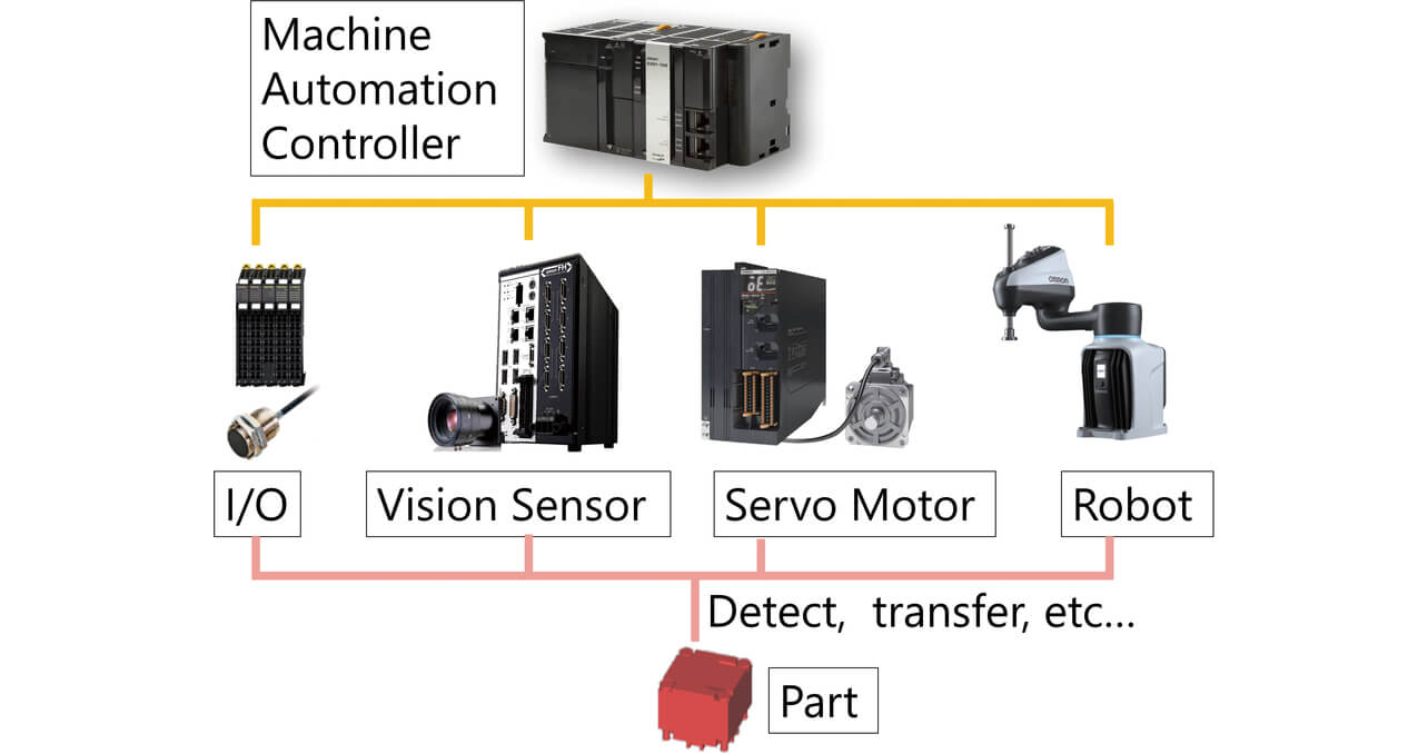
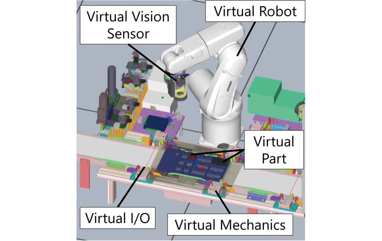
Before virtualization technology became widespread, production facility development typically relied on real machines only. To reduce the required man-hours for production facility start-up, OMRON incorporated production facility virtualization technology into its FA-integrated development environment, Sysmac Studio. Fig. 1 illustrates a typical configuration of a complete production facility, which includes the following components: an I/O for sensor control, an image sensor (Vision Sensor), a servomotor for peripheral device control, and a robot. These components perform detection, transfer, and other workpiece/parts-related tasks. To achieve the virtualization of these components, we developed five virtual modules: virtual I/O, virtual vision sensors (virtual image sensors), virtual mechanics (virtual peripheral device), virtual robots, and virtual parts (virtual workpieces). Fig. 2 shows an example of the achieved production equipment virtualization.
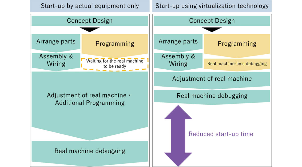
We found that through the active use of our conventional technology, start-up man-hours could be reduced by 56% compared to relying exclusively on real machines1). Fig. 3 compares two development processes leading to production facility start-up: one reliant exclusively on physical machines and the other involving virtualization technology.
2.2 Challenges to our conventional virtualization technology
Among the components of production facilities, peripheral devices exhibit an exceptionally wide variety. The mechanical mechanisms constituting our conventional virtual mechanics support 13 general-purpose types, including linear motion mechanism, rotary motion mechanism, and air cylinder. These types are defined as creatable mechanisms. However, peripheral devices are often custom built to suit users’ production facilities. Custom-made peripheral devices may contain mechanisms not supported by the 13 general-purpose types. More specifically, these mechanisms include electric cylinders and chucks, which have varying detailed settings depending on the manufacturer, and clamping mechanisms that require simulations of physical phenomena. Our conventional virtualization technology cannot reproduce peripheral devices containing such mechanisms as 3D objects in a virtual space. If a production facility contains even one peripheral device that cannot be reproduced as a 3D object, it becomes impossible to 3D simulate the facility in a virtual space. Consequently, reliance on real machines becomes necessary to debug or adjust such peripheral devices, reducing productivity. It is crucial to reproduce these peripheral devices as 3D objects to achieve a 3D simulation of an entire facility in a virtual space.
3. Development of Custom Mechanics
To address the challenge described in Section 2 regarding our conventional technology, we focused on developing a function that enables users to create virtualization models of any mechanism. Suppose the user could freely modify manufacturer-specific setting items and values, define their original mechanisms, including physics simulations, and integrate them into their virtualization models. This advancement would allow the user to 3D simulate an entire facility in a virtual space, effectively solving the challenge mentioned above. We refer to a module with this function as Custom Mechanics, distinguishing it from virtual mechanics, which supports the 13 types of general-purpose mechanical mechanisms.
The critical elements in the development of Custom Mechanics are movable-parts connection joints. The user must simulate physical phenomena using physics simulation technology to reproduce joint motions as simulations. Subsection 3.1 presents a solution to the challenges in that development. Subsection 3.2 discusses a technology that synchronizes Custom Mechanics with the pre-existing virtual modules to enable the 3D simulation of an entire facility in a virtual space. Subsection 3.3 describes a technology with which the user can easily configure the complicated system, including Custom Mechanics.
3.1 Developing movable-parts connection joints
To reproduce as a 3D object a mechanism that incorporates movable parts interconnected according to physical phenomena, the user needs to perform a physics simulation of the interconnection of the movable parts to establish constraints on their relative motions. Sysmac Studio relies on the PhysX real-time physics engine provided by NVIDIA for physics simulations. PhysX comes with a D6 Joint predefined to control the x-, y-, and z-axes and their rotations separately from each other2). However, the D6 Joint does not directly represent the mechanisms of the joints of mechanisms and hence, with its default interface, cannot serve as the Custom Mechanics joint intended for quick and easy configuration. Then, to provide intuitively user-friendly Custom Mechanics joints, we defined joints referring to the classification of mechanisms presented in a reference (“Karakuri Designs”), a collection of mechanism formulas for mechanism designs3). Based on their definitions, we customized the D6 Joint’s interface to develop our original group of joints listed below in Table 1:
| Joint | Descriptions |
|---|---|
| Fixing joint | A connection method for fixing two movable parts |
| Hinge joint | A method of connecting two movable parts via a hinge joint |
| Ball joint | A method of connecting two movable parts via a ball joint |
| Slider joint | A method of connecting two movable parts in a linear direction |
| Revolute joint | A method of connecting two movable parts rotatably about a single axis |
| Parent-child joint | A connection method based on the parent-child relationship between two movable parts |
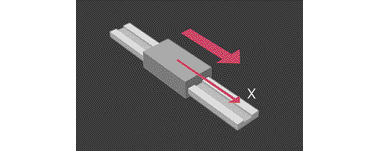
Fig. 4 illustrates the motion of the slider joint as an example of our original joints. This joint was created by locking all translational and rotational motions of the D6 joint, except those with respect to the x-axis. Similarly, the other joints, apart from the parent-child joint, were created by locking the specific motion directions of the D6 joint.
The parent-child joint was developed to reproduce as 3D objects mechanisms, such as an electric chuck mechanism, which combines the motion axis-based position control of a programmable logic controller (PLC) with a joint mechanism. In this mechanism, one movable part is set into motion by PLC motion control, and its motion is followed by the other movable part containing a joint. These two movable parts rely on a parent-child relationship between them to have their relative coordinates updated. When each part of the mechanism is simply set into motion, the part position to be followed is updated in the motion cycle next to the current one. Consequently, when the mechanism is viewed as a whole, a delay occurs with respect to the initially predicted position. To address this issue, we ensured that the following sequence of operations occurs on a mechanism-by-mechanism basis: updating the movable parts’ positions according to the PLC’s motion-axis command value, performing a physics simulation of the joint using the freshly updated position data, and determining the 3D world coordinates of the whole mechanism based on the simulation results. As a result, it has become possible to simulate the motions of mechanisms containing a parent-child joint in sync with those of other mechanisms. These technical improvements led to the fruition of Custom Mechanics, significantly expanding the range of virtualizable equipment.
3.2 Achieving inter-component synchronization for enabling 3D simulations of whole facilities
Fig. 5 shows the overall system configuration of Sysmac Studio:
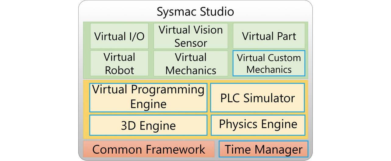
(Green–Objects to be virtualized; Yellow–Virtualization engines;
Orange–Software platforms)
The common framework provides the foundation for making all the virtualized modules function on a single piece of software. The time manager manages the execution timing of each engine. Its details will be presented later. Then, the virtual programming engine (virtual programming environment) executes programs for production facility control and simulation. The PLC simulator simulates the operation of the real PLC. The 3D engine manages 3D model geometry data of production facilities in their entirety, provides 3D display functions, and checks models for interference. The physics engine performs computational operations for gravity or physics simulations. The modules that serve on the 3D engine as the virtualized forms of the production facility elements of robots, peripheral devices, I/O devices, image sensors, and workpieces are the virtual robot, virtual mechanics (virtual peripheral device), virtual I/O, virtual vision sensors (virtual image sensors), and virtual parts (virtual workpieces). This time, we added a virtual Custom Mechanics (virtual custom mechanical mechanism) module. Note that the modules modified then by adding an interface or otherwise are highlighted with a blue box.
To provide the virtual environment in Fig. 5, including Custom Mechanics, all the elements in the system must function synchronously with each other. If the system’s functions are mutually out of sync, each simulation run yields different results from those of others. Consequently, in such cases as when the Custom Mechanics module is used to pick workpieces flowing on the conveyor and place them on another conveyor, problems occur, such as inaccurate picking. Besides, failure to achieve high-speed inter-component synchronization results in the problem of unsmooth rendering on the 3D display screen.
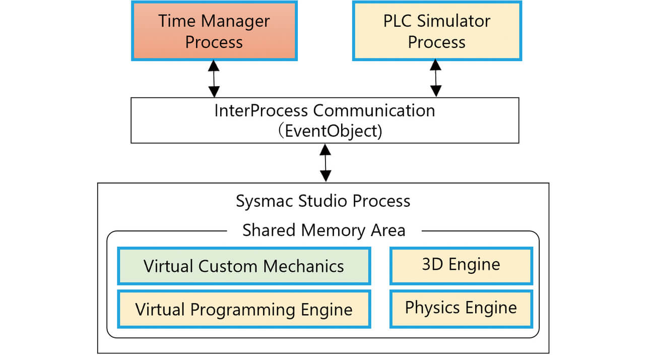
What it takes to solve these problems is to achieve high-speed synchronization between Custom Mechanics and the pre-existing modules of the system. Fig. 6 shows the relationship between the processes, i.e., the run units of the modules in the subsystem containing Custom Mechanics extracted from the system shown in Fig. 5. To attain high-speed inter-process communication, we achieved inter-process synchronization, using EventObject in the Windows operating system. As a result, an inter-process communication speed of approximately 0.02 ms became available, enabling smooth monitoring of motions on the 3D display screen even in cases where Custom Mechanics is involved.
In addition, the data exchange speed between different elements in the memory space in the Sysmac Studio process also poses a challenge to 3D simulations of the gravity or collisions between Custom Mechanics joints and workpieces as closely as possible to real-time actions. Sysmac Studio uses Shape Script, a C#-based general-purpose programming language for virtualization, to reproduce workpiece motions as simulations in a virtual space. Shape Script, implemented in the virtual programming engine, reads and writes values to and from the PLC simulator variables. As such, Shape Script requires high-speed communication with other components in the Sysmac Studio process. High-speed communication between the virtual programming engine and the other components is provided using the .NetRemoting framework for high-speed communication between different elements in the memory space provided by the operating system1,4). In Custom Mechanics, a dedicated interface for Shape Script to synchronize mechanism motions is provided to use these communication frameworks and achieve 3D simulations close to real-time actions.
To ensure the system-wide management of inter-component synchronization involving Custom Mechanics for the whole system, we expanded the time manager1), which manages the timing of each component. Fig. 7 shows the time chart for the simulation time synchronization across the whole system.
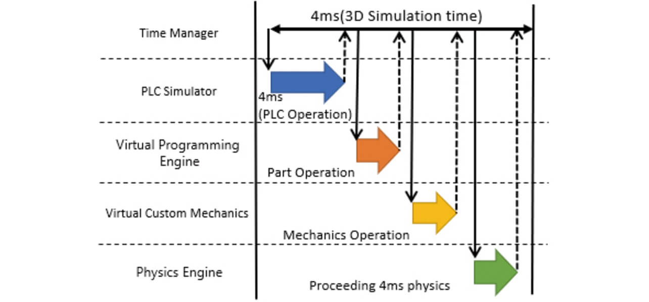
By allowing the time manager to manage mechanism motions in virtual Custom Mechanics, we achieved successful operational synchronization between the Custom Mechanics and pre-existing virtual modules.
3.3 Solving the usability issues in configuring Custom Mechanics
This subsection discusses the challenges in enabling user-friendly configuration of Custom Mechanics and our solutions to them.
3.3.1 Developing a snap function for easy joint position setting
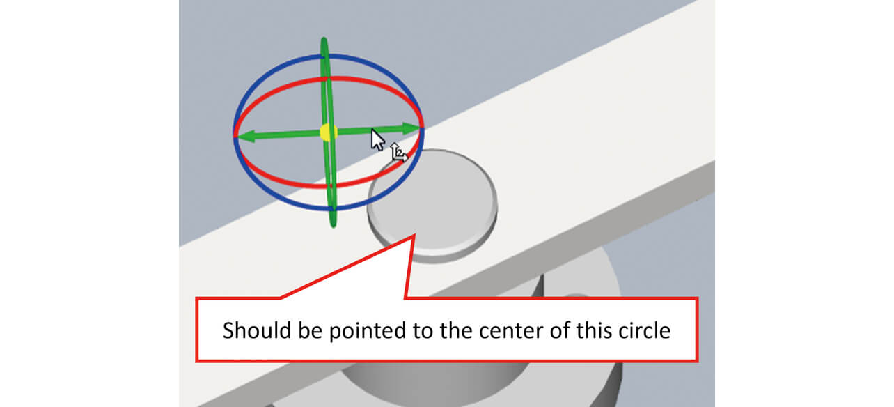
As mentioned above, we used physics simulations to reproduce Custom Mechanics joint motions as simulations. Physics simulation cannot be performed accurately without precisely determining the joint position between the movable parts involved. As shown in Fig. 8, a joint position can be set using mouse operations. However, some target positions may not appear on the screen. In addition, the accuracy of point movements varies depending on the user’s mouse operations. These factors make it challenging to set joint positions accurately.
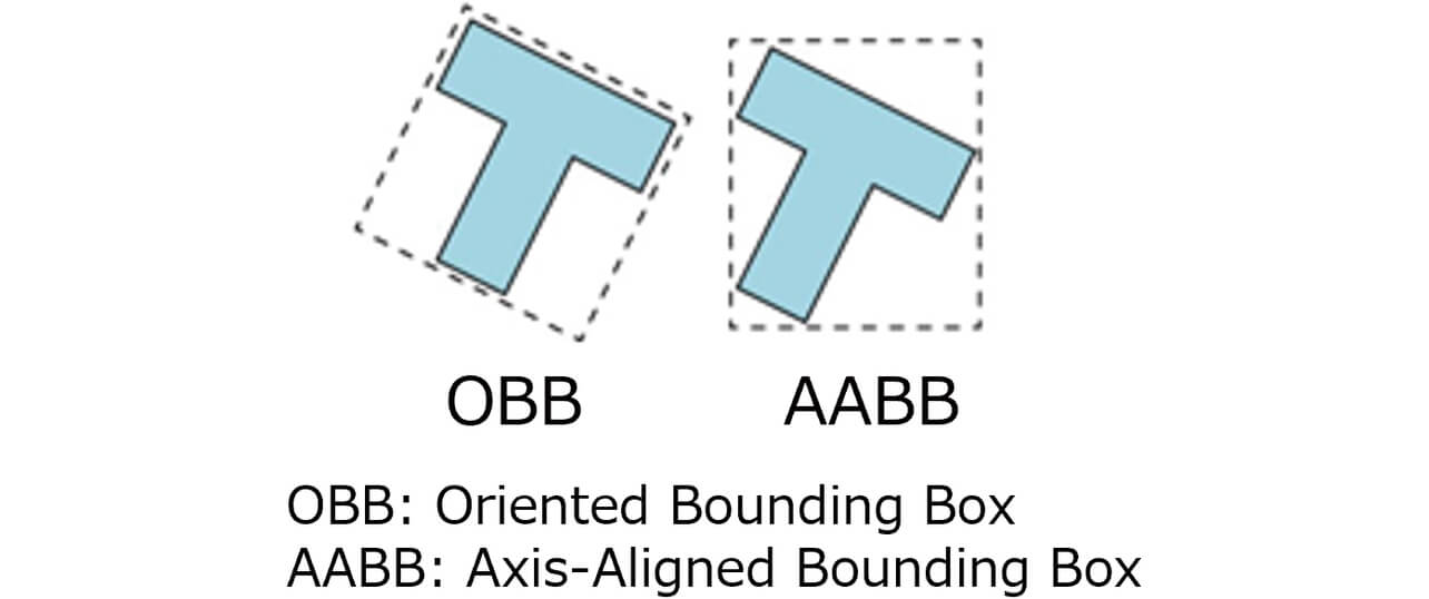
As a solution to this problem, we developed a snap function. When the user clicks and chooses a specific 3D object and moves the mouse cursor onto another 3D object, this function indicates feature points close to the mouse cursor, such as the two ends of a nearby edge or the center of gravity of a nearby face, so that the user can move the target object to such points by clicking on them. The face nearest to the mouse cursor must be searched to allow the snap function to make candidate destination points appear on the screen. However, this search for the snap destination point requires much computation, affecting the user’s mouse operation or otherwise reducing performance. To reduce the amount of computation, we chose to simplify 3D objects using cuboids. Fig. 9 shows two simplification methods available: OBB and AABB. Considering that our point of interest related to operability, we selected the AABB method, which has an edge in response speed.
The method that applies AABB for simplification is used to identify the foremost object from among the objects in the area the mouse cursor indicates. This method of identifying the foremost object is established as the sequence of the following steps: creating a ray that connects the camera to the mouse cursor and obtaining the object closest to the camera from among the 3D objects intersected by the ray. Then, each internal geometry data constituting the identified 3D object is bounded with a cuboid for a search to identify the foremost face. The information of the two ends of the nearest edge or the center of gravity of the nearest face is obtained from the identified face to render these points as the Snap destinations on the screen.
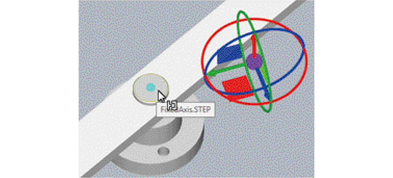
We added an improvement enabling computational processing in the background to achieve further performance enhancement. Computations are always performed for the point where the mouse cursor is. New computations occur when the mouse cursor moves. When the mouse cursor is moved too fast, no snap destination appears on the screen because of the processing performed in the background. However, as the mouse cursor is brought closer to the snap target and is moved slower, the snap destination point or points appear on the screen. This improvement was achieved as a result of designing it with a focus on the user’s method of mouse operation. More specifically, the improvement was designed considering the human tendency to move the mouse quickly until near the target coordinates and slowly near the target position. Fig. 10 shows how to specify a joint position using the snap function developed through these technical efforts. When the mouse cursor is moved closer to the target position after selecting a joint and going into snap mode, a light blue point appears on the screen. When this light blue point is clicked, the joint moves to it.
Thus, we developed an operationally user-friendly, intuitively natural snap function, enabling accurate positioning of joint positions necessary for physics simulations.
3.3.2 Developing a motion setting function that makes it simpler to define the motions of multiple movable parts
Electric chucks are among the critical mechanisms desired to be reproduced as Custom Mechanics objects. Intended to grip an object with multiple jaws, an electric chuck is required to get multiple movable parts into motion as a set. To serve this purpose, a standard electric chuck has a distinctive function known as the motion number function5). This function bundles the speeds, positions, and other motion features of multiple movable parts into a group of settings in advance and assigns a number to that group of settings. For example, SMC’s step motor controllers, which can control electric chucks, perform operation control according to step-data instructions, which are collections of motion instructions for multiple movable parts. To enable motions of multiple movable parts in Custom Mechanics according to step-data instructions, one must define the motion of each movable part in Shape Script. However, a typical Custom Mechanics object must have ten-odd numbers of step data defined. An extremely complicated script would be necessary to manage that many step data. Besides, the control program must be modified to associate these data with their corresponding motion number specification PLC variables, posing another barrier to the user.
Accordingly, we developed a new function equivalent to the electric chuck motion number function. This new function can bundle the motion settings for multiple movable parts into an easily manageable group. This function automatically and internally calculates speeds and positions based on motion settings, associating these values with motion number specification PLC variables. In addition, we provided a table-format user interface shown in Fig. 11, on which the user can intuitively make these motion settings.
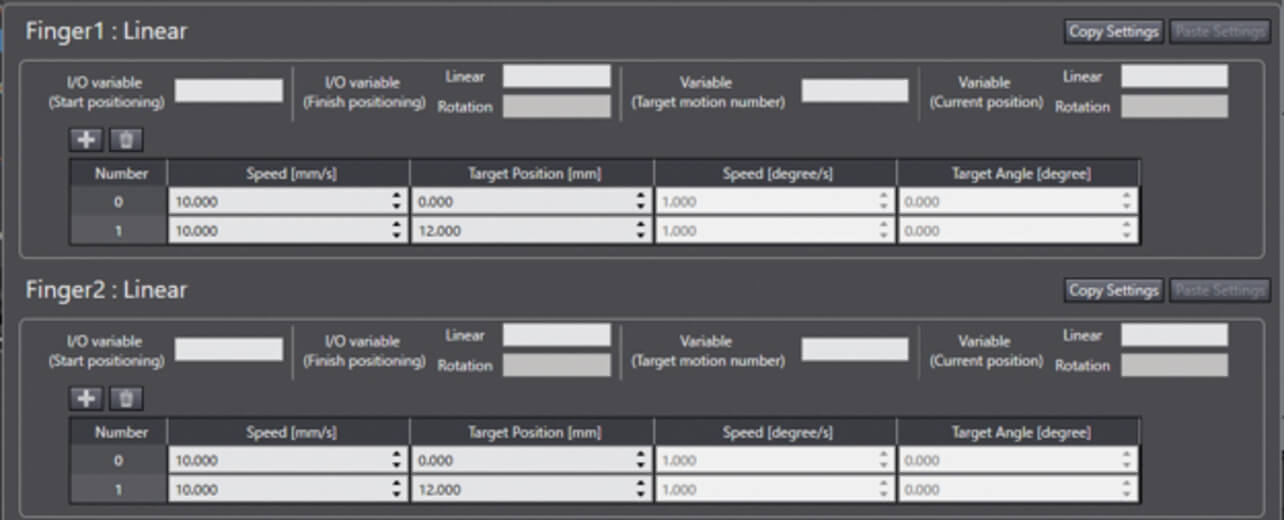
The Motion Settings screen allows the user to select a linear, rotational, or linear-rotational motion direction for each movable part of a Custom Mechanics object and preset up to 64 motions corresponding to each motion direction. Table 2 shows the contents of the settings to be made for each motion direction.
| Motion direction | Motion setting content |
|---|---|
| Linear | The linear speed [mm/s] and target position [mm] are to be specified to indicate that the movable part linearly moves at the specified linear speed [mm/s] until reaching the target position [mm]. |
| Rotational | The rotational speed [degrees/sec] and target angle [degree] are to be specified to indicate that the movable part rotates at the specified rotational speed [degrees/sec] until reaching the target angle [degree]. |
| Linear-rotational | The linear speed [mm/s], target position [mm], rotational speed [degrees/sec], and target angle [degree] are to be specified to indicate that the movable part linearly moves at the specified linear speed [mm/s] until reaching the target position [mm] and then rotates at the specified rotational speed [degrees/sec] until reaching the target angle [degree]. |
Each movable part must be assigned with the following setting parameters: start positioning I/O variable, finish positioning I/O variable, specify motion number variable, and get current value variable. Table 3 shows the descriptions of these variables. While the start positioning I/O variable is on (True), each movable part moves at the speed of the motion number specified by the specify motion number variable toward the target position of the motion number. Then, when the movable part stops at the target position, the finish positioning I/O variable turns on. The current values of the movable part are always written out to the get current value variable. The variables of the controllers or the I/O signals of the robot can be assigned to the above variables. As explained in Subsection 3.2, the fetching and writing of these variables’ data are managed to occur in sync across the whole system.
| Variable | Descriptions |
|---|---|
| Start positioning I/O variable | While on, this variable sets a movable part into motion according to the settings of the specified motion number. |
| Finish positioning I/O variable | This variable turns on when the movable part reaches the target position. |
| Specify motion number variable | This variable specifies the motion number for the movable part from among up to 64 user-settable motions. |
| Get current value variable | The current position of the movable part is always written out to this variable. |
Fig. 12 shows typical motions of an electric chuck with two jaws/movable parts, with two motion setting values assigned to each jaw. The motions are defined so that the chuck closes with Motion Number 0 and opens with Motion Number 1. To define these motions, the user only has to fill in the necessary items on the Motion Settings screen.
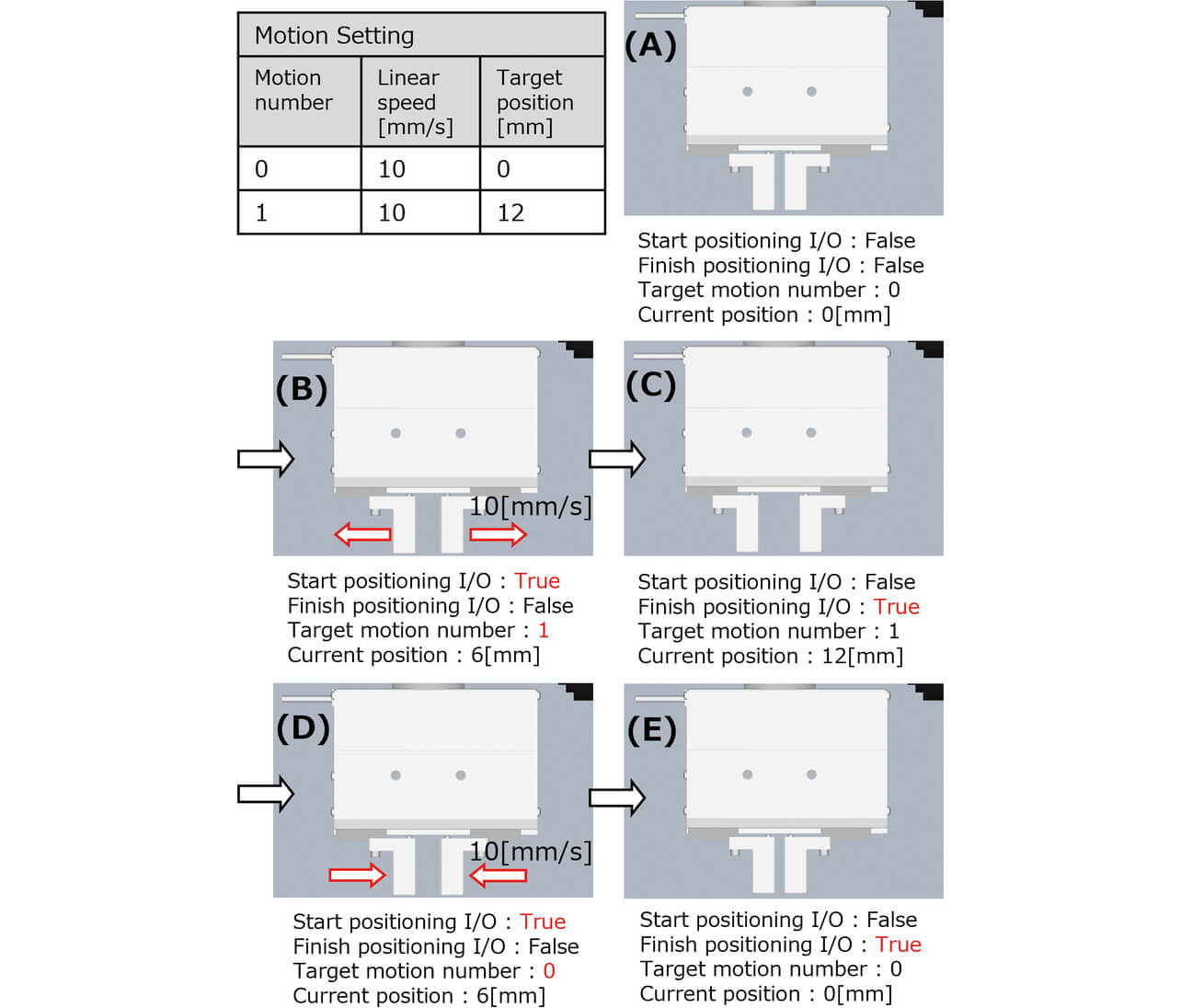
Fig. 12(A) shows the initial state where the chuck is closed. When the specify motion number variable is set to the value “1,” and the start positioning I/O variable is switched to the value of “TRUE,” as shown in Fig. 12(B), the movable parts move toward a target position of 12 mm at a linear speed of 10 mm/s according to the motion setting for Motion Number 1. When the movable parts reach the target position for Motion Number 1, the start positioning I/O variable takes the value of “FALSE,” as shown in Fig. 12(C). Meanwhile, the finish positioning I/O variable takes the value of “TRUE.” Consequently, the chuck goes into the open position. Then, when the specify motion number variable is set to the value of “0,” and the start positioning I/O variable is switched to the value of “TRUE,” as shown in Fig. 12(D), the movable parts move toward a target position of 0 mm at a linear speed of 10 mm/s according to the motion setting for Motion Number 0. When the movable parts reach the target position for Motion Number 0, the finish positioning I/O variable takes the value of “TRUE,” putting the chuck in the closed position, as shown in Fig. 12(E).
As explained in this subsection, we developed a motion setting function that bundles together motions of multiple movable parts and puts them into motion as a single group. With this function, the user can now easily define complicated motions of Custom Mechanics objects.
4. Verifying the effectiveness of Custom Mechanics
Aiming to verify the effectiveness of the virtualization technology made available by Custom Mechanics, we built a door switch mounting system integrated with a robot and Custom Mechanics as an example of equipment containing all the technical elements discussed herein.
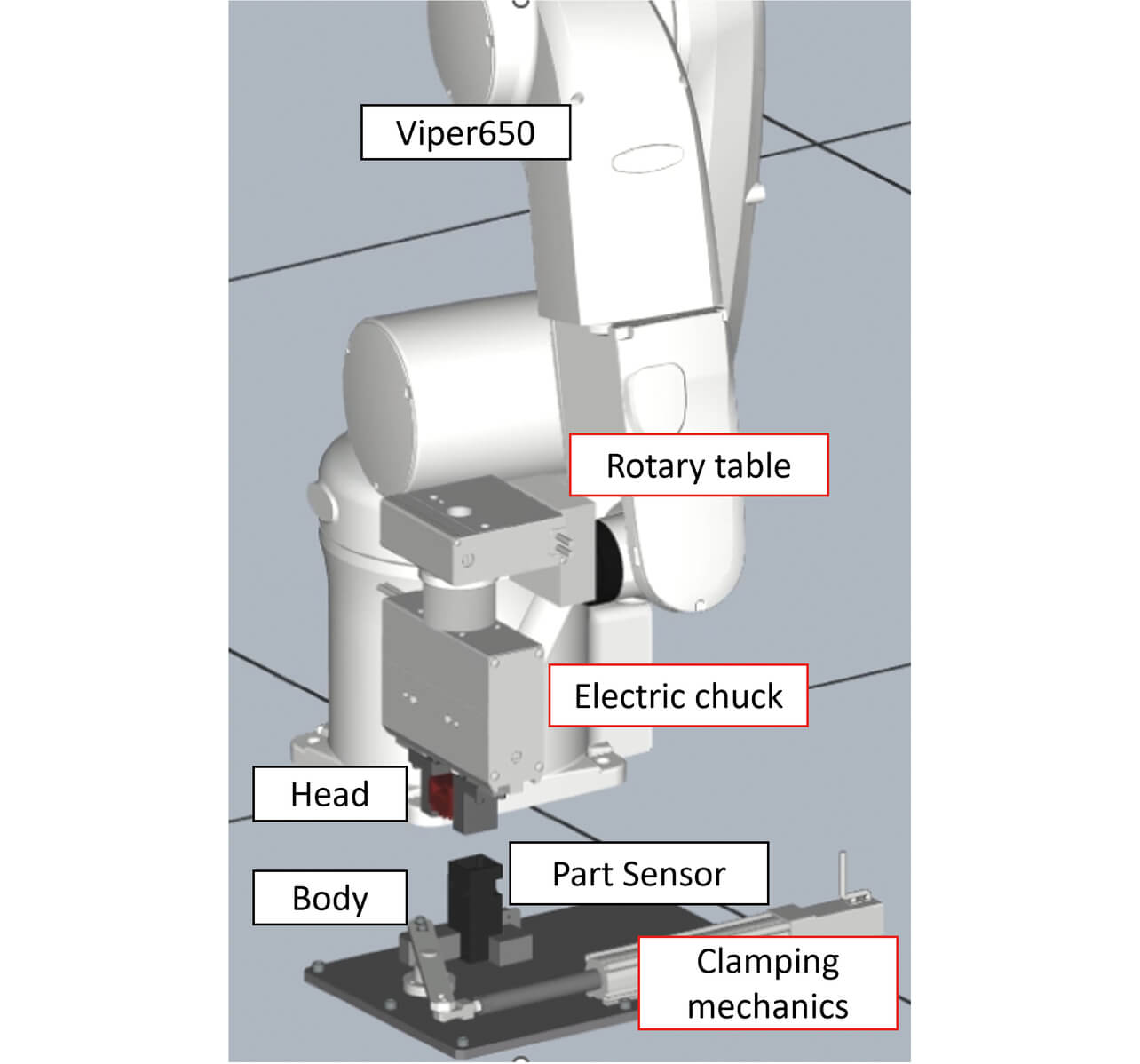
In this door switch mounting system, the Viper 650 vertical multi-joint robot transfers the body and head of a door switch in order and mounts the door switch’s head onto its body. At the destination, a clamping mechanism holds down the body in position so it can be mounted with the head. In the system, the rotary table and electric chuck attachments to the end effector of the Viper 650 and the clamping mechanism for holding the body down are reproduced as Custom Mechanics objects. Fig. 13 shows the configuration of the system used for verification. Table 4 provides the descriptions of the individual mechanisms.
(Red boxes: Custom Mechanics objects)
| Item | Descriptions | |
|---|---|---|
| Viper 650 | A PLC-controlled vertical multi-joint robot. | |
| Body (Door switch) | A workpiece to be transferred, on top of which the Head is to be mounted. | |
| Head (Door switch) | A workpiece to be transferred and mounted on top of the Body. | |
| Part Sensor | A sensor that detects that the workpiece is held down in the fixation position. | |
| Custom Mechanics objects |
Rotary table | A Custom Mechanics object that turns to adjust the end-effector position. |
| Electric chuck | A Custom Mechanics object that grips the workpieces. | |
| Clamping mechanics | A Custom Mechanics object that holds down the Body to mount the door switch’s Head on it. | |
This verification covered the processes from mechanism design through real machine building and control design to control debugging, including overall verification, for the door switch mounting system. We recorded the man-hours spent on these processes for comparison with and without our new virtualization technology. Fig. 14 shows the results of the comparison.
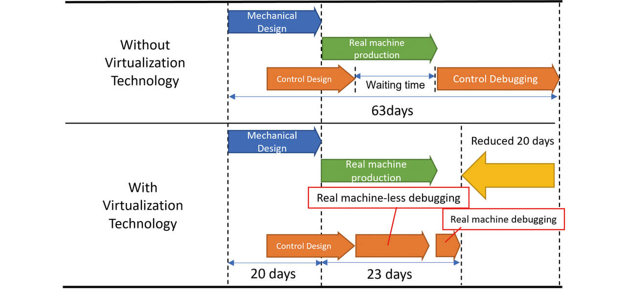
Without the help of the new virtualization technology, the start-up took 63 days as shown in Fig. 14. Conversely, the required time was reduced to 43 days with the help of the new virtualization technology. Thus, an approximately 32-percent reduction of start-up man-hours was achieved with this technology.
When the new virtualization technology was not used, a waiting time occurred because control debugging remained impossible after the mechanism design stage started until all the real machines were ready for use upon completing the real machine-building stage. On the contrary, when the new virtualization technology was used, the whole system was completed in a shorter time because the control debugging stage proceeded simultaneously with the real machine-building stage without waiting for the latter to complete.
The use of any real machine for the teaching process in control debugging leads to an increase in man-hours because the robot must be operated at a lower speed to avoid equipment damage due to interference. Meanwhile, the use of our new virtualization technology enables the high-speed operation of virtual robots in a virtual space, thereby reducing teaching time. In addition, the final adjustments with the real machines required almost nothing but checks and fine-tuning, reducing the hours worked with the real machines. Consequently, the overall man-hours for control debugging were also reduced.
Moreover, programs created using our virtualization technology and debugged without using any hardware can be applied as they are to real machines. Hence, unlike conventional virtualization simulations, these programs need no additional programming at the start-up of real machines, thereby helping to reduce the lead time before starting the verification work with real machines.
5. Conclusions
This paper discussed how to implement and apply Custom Mechanics incorporating physics simulation technology to solve the problem that 3D simulation-based facility pre-verification is impossible when any equipment contains even a single mechanism unsupported by our conventional technology.
We achieved successful operational synchronization between the Custom Mechanics module and the pre-existing virtual modules for 3D simulations of various movable-parts connection joints or facilities in their entirety. Besides, we solved the usability issues involved in the use of Custom Mechanics, including the joint position Snap function or the motion setting function.
As applied to door switch system manufacturing, our new technology was observed to cut the man-hours by 32% and was verified for effectiveness. As such, this technology enables short-term start-up of production facilities, thereby contributing to timely product launches.
Moving forward, we intend to advance our virtualization technology further to achieve the virtualization of gears, cams, and other mechanisms that require additional intrinsic-parameter settings and are yet to be virtualized as Custom Mechanics. Alternatively, we would like to avidly introduce technologies, such as finite element method technologies not incorporated yet in Sysmac Studio, to enhance the applicability of virtualization to a broader range of facilities and equipment, including flexible objects.
References
- 1)
- H. Shimakawa and S. Iwamura, “Production Equipment Virtualization Technology by Integrated Development Environment for Factory Automation,” (in Japanese), OMRON TECHNICS, vol. 53, no. 1, pp. 8-16, 2021.
- 2)
- PhysX Joints, “NVIDIA PhysX SDK 3.4.0 Documentation,” https://docs.nvidia.com/gameworks/content/gameworkslibrary/physx/guide/Manual/Joints.html (accessed Jan. 13, 2023).
- 3)
- H. Kumagai, A Must-Have Collection of Mechanism Formulas for “Karakuri Designs” - Starting Simplified Automation with Zero Prior Knowledge. Nikkan Kogyo Shimbun, Ltd. (in Japanese), 2017.
- 4)
- Microsoft, “Outline of NET Remoting Framework,” (in Japanese), https://learn.microsoft.com/ja-jp/previous-versions/msdn/architecture-center/cc440094(v=vs.71) (accessed Jan. 13, 2023).
- 5)
- SMC, “Controller (Step-Data Input Type) JXC51/61 Series,” (in Japanese), https://ca01.smcworld.com/catalog/Electric/mpv/s100-136-JXC51-61/data/s100-136-JXC51-61.pdf (accessed Feb. 6, 2023).
The names of products in the text may be trademarks of each company.