


Fast Motion Planning Technology for Vertical Articulated Robot
- Robot
- Path Planning
- Trajectory Planning
- Trajectory Optimization
- Collision Checking
In recent years, due to soaring labor costs and the spread of a new type of coronavirus, there has been an increasing demand to save labor at the production sites. However, the need for industrial robots, especially vertical articulated robots, has been increasing as one of the laborsaving measures, but they have not been widely used because of the many person-hours and expertise required to generate the motions of the robots that can achieve high productivity.
In this study, we developed a fast motion planning technology for a vertically articulated robot. The motion planning technology consists of two technologies: path planning and motion acceleration. In the former, we reduced the processing time for path planning to 100 ms, which is several seconds per motion in conventional technology, by selecting a context-specific algorithm and fast collision checking. In the latter, by optimizing the acceleration parameters and path correction to reduce the inertia on the robot joints, the tact time was improved by about 20% compared to the robot’s default parameters. To confirm the effectiveness of these technologies, we built a bin-picking system. It works in the 3 seconds as much as a person’s tact time without any robot motion generation by the user.
1. Introduction
In recent years, due to soaring labor costs and the spread of a new type of coronavirus, there has been an increasing demand to save labor at the production sites. Studies are vigorously underway to introduce industrial robots as a method of saving labor. Needs are mounting for vertically articulated robots with a wide operating range and a high degree of freedom of motion to perform tasks in place of or in collaboration with human operators. In reality, however, production sites and, in particular, small and medium-sized companies, are lagging behind in introducing robots. The main factors considered responsible for this problem include the time-consuming robot motion generation and higher degrees of difficulty in motion generation tasks1).
For an industrial robot to perform a task, its motions must be generated by performing the so-called teaching task for setting the position and posture for the robot to move and the parameter adjustment task for motion speed and other settings. These are both time-consuming tasks that involve working on actual robot operations by trial and error. Moreover, both these tasks require expertise and skills, including joint angle settings for robot control and torque considerations.
Accordingly, we developed an automatic robot motion generation technology that automates the position-posture setting and motion parameter adjustment tasks for vertically articulated robots. This technology allows users not well versed in robots to introduce robots into their production sites. Besides, our proposed technology can generate motions at a computational time of 100 ms or less per motion; hence, the technology supports bin-picking and other applications that require motion generation as the need arises.
In what follows, Section 2 presents the challenges to motion generation by industrial robots and the development targets, Sections 3 and 4 describe the automatic robot motion generation technology developed, Section 5 explains a bin-picking application implemented based on the development results obtained, and Section 6 presents the conclusions and future prospects.
2. Challenges to robot motion generation and technology development targets
2.1 About robot motion generation
A vertically articulated robot is controlled by the rotation angle of each joint servomotor. A robot’s condition, which consists of a set of rotation angles of the respective joints, is called a posture. In its most simplistic form, robot motion generation can be achieved by specifying the following two postures: one being an initial posture (current posture) for the robot to start a motion and the other being a goal posture for it to perform a task. This form of control method is called point-to-point (PTP) control. However, a PTP-controlled motion simply connects the two postures by linear interpolation and may collide with some obstacle between the initial posture and the goal posture.
An alternative control method is available and is used to specify detailed intermediate postures between the initial posture and the goal posture for a robot to perform precise motions. This form of control is called continuous-point (CP) control. A set consisting of a robot’s initial and goal postures given for CP control and the intermediate postures in between is called a path. Fig. 1 shows the differences between a PTP-controlled motion and a CP-controlled motion.
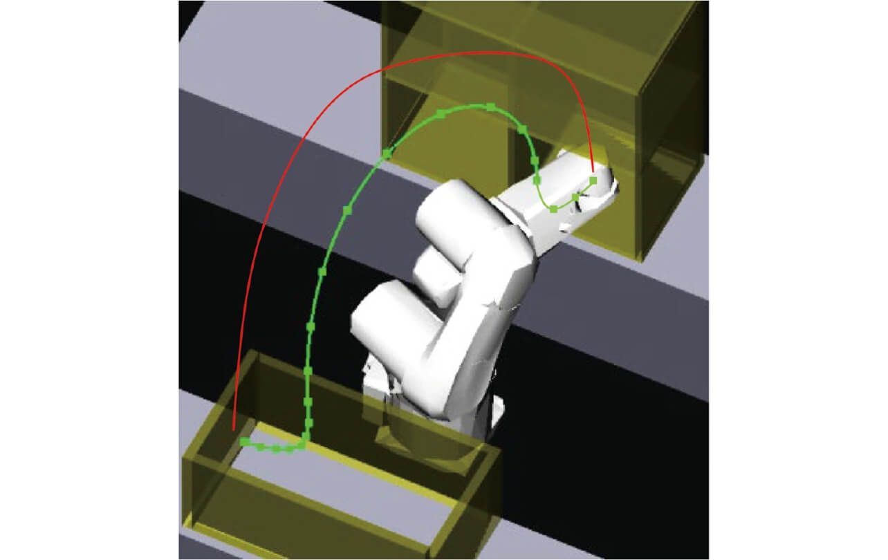
Moreover, for the robot to perform an actual motion, it is also necessary to specify how the set path should be executed over time. This change over time can be made to occur by controlling motion parameters, such as servomotor velocity and acceleration. Such a path with given motion parameters to be executed along the time base is called a trajectory. In other words, motion generation of a robot means trajectory generation by the robot.
2.2 Challenges to path generation
A task generally known as teaching is performed to generate paths for performing CP control. In this task, a human operator manipulates a real robot, using a robot operating device called a teaching pendant (TP), to register postures constituting the path one by one. Postures given during teaching are also known as teaching points.
Generally, the number of teaching points necessary to use a robot as production equipment ranges from several tens to several hundreds, which may vary depending on the complexity and amount of the task. For accurate teaching point setting, the robot must be verified for its postures by reducing its motion speed or stopping it. Therefore, teaching faces the challenge of a large number of person-hours.
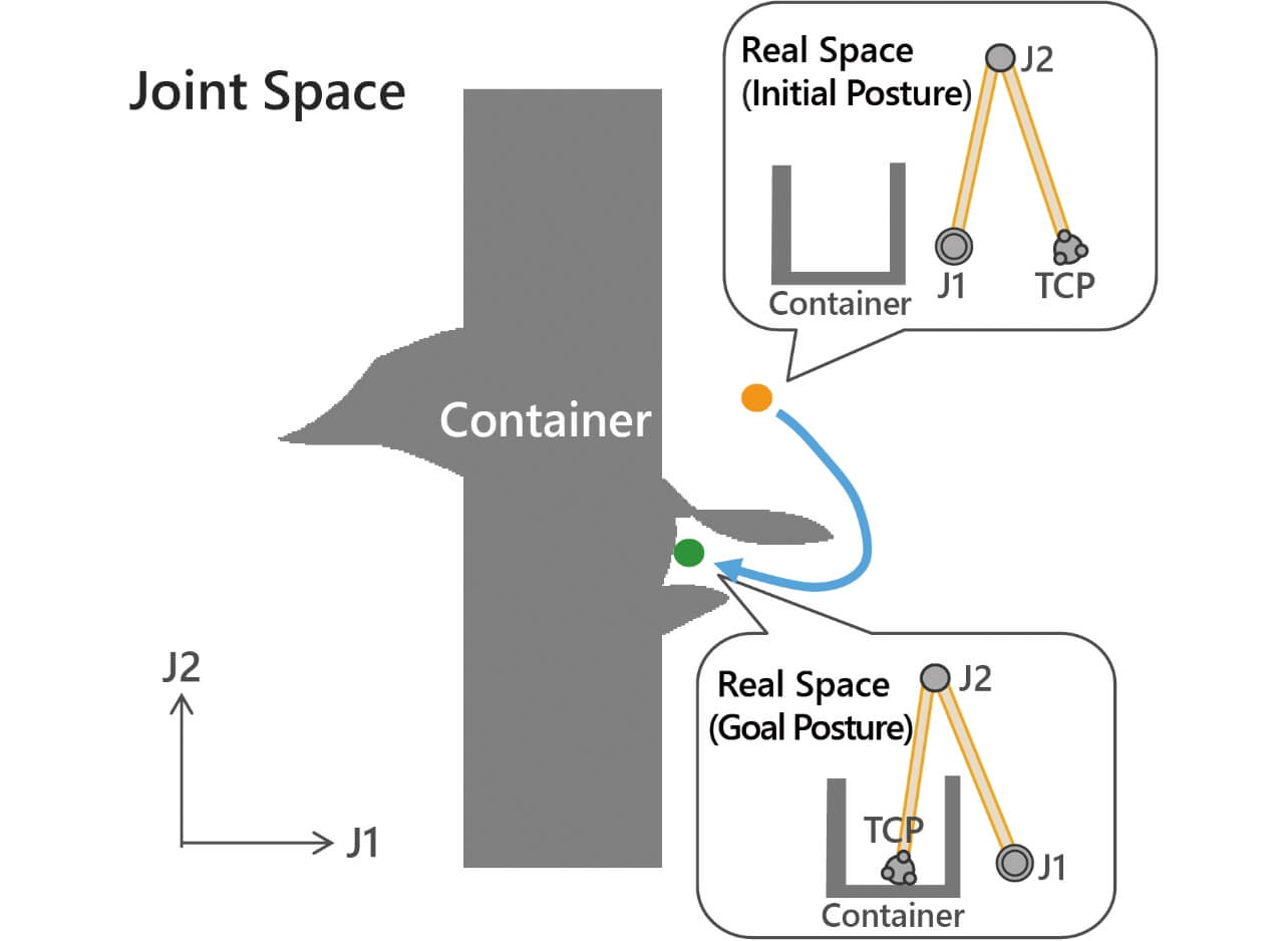
Another challenge is that considerable skill is required for robot manipulation to make a robot assume postures given as teaching points. This challenge arises from the gap between the human spatial recognition based on an orthogonal coordinates system (real space) consisting of three axes, a longitudinal axis (X), a transverse axis (Y), and a vertical axis (Z), as well as the robot’s operation parameter, in other words, its joint rotation angle (joint space). Fig. 2 explains this challenge using a 2-DOF robot moving on a plane as an example.
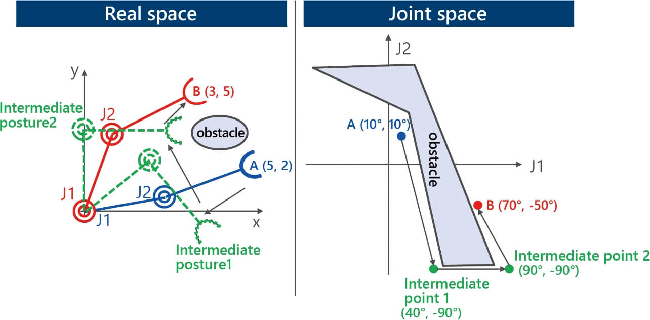
To move from the initial posture A to the goal posture B in real space while avoiding obstacles, the robot must assume intermediate postures 1 and 2 on the way to avoid collisions. Humans can intuitively estimate the positions of the intermediate postures in real space. These positions, however, do not convert readily into joint angles for controlling the robot. The TP has a function called orthogonal jog operation to translate the robot end-effector relative to real-space coordinates, which brings the robot manipulation closer to a certain degree to human intuition. However, this translation of the end-effector by orthogonal jog operation is performed by the robot controller that controls each joint’s movement. Hence, the user has no control over the movement of the robot’s parts (elbow/shoulder) other than the end-effector. Therefore, an attempt to rely entirely on orthogonal jog operation for teaching results runs the risk of causing collisions between the robot and its surrounding environment. Besides, the real and joint spaces are in a non-linear relationship, which means the existence of regions that are continuous in the real space but discontinuous in the joint space. The robot controller’s computational outputs become indefinite joint values in such regions, causing the robot to perform redundant motions or stop moving. Thus, an attempt to move the robot over a long distance with the orthogonal jog operation often results in failure to obtain the movement as desired by the user. Accordingly, in actual teaching, the user must depend on trial and error to change each joint rotation angle until obtaining the posture close to the desired teaching point to perform a precise alignment task with the orthogonal jog operation.
It follows from the above that the current form of robot teaching is highly burdensome on users because it must be worked on through trial-and-error cycles by a skilled operator based on intuition and experience.
2.3 Challenges to trajectory generation
For a robot to be used as production equipment, it is necessary that a path generated by teaching be executed in time to meet the user’s desired takt time. For this purpose, a high-speed trajectory must be generated by adjusting the joint rotation velocity between the intermediate postures on the path.
The robot’s joint rotation velocity is controlled by the parameters of the maximum velocity value and acceleration. In principle, when these parameters are set to a high value, fast motion is obtained. However, these parameters must be set to the appropriate value that is not excessively high. Otherwise, the torque load on each joint servomotor would become high and cause the safety device to trip and stop the robot.
As shown below by Equation (1), the torque is affected by the mass and the inertia. Hence, to obtain the optimal parameter values, the user’s consideration must extend to the mass and posture of the hand mounted on the robot or those of the workpiece grasped by the hand.

- τ: Load (torque)
- M (
 ): Mass-related matrix
 - V (,
 ): The vector representing the centrifugal and Coriolis force terms
 - F (): The vector representing the friction force term
- G (): The vector representing the gravity term
Therefore, if the required takt time cannot be met using the recommended values, the user must adjust the parameters by trial and error while manipulating the real robot. As is the case with teaching, this task is a skill-demanding and time-consuming one, in other words, a burdensome task for the user, posing a challenge.
Another challenge is posed by cases that require path readjustments besides motion parameter readjustments to achieve a short takt time. For example, in some cases, the loads on a robot’s joints become smaller with the robot operated in an arm-retracted posture rather than an arm-extended posture, thereby allowing the robot to perform the intended motion at a higher speed in a shorter total motion time.
From the above, it follows that the challenge of adjusting both the motion parameters and the path by trial and error must be addressed to generate a trajectory for the robot to achieve high productivity.
2.4 Technology development targets and evaluation environment
We developed an automatic path generation technology and an automatic motion acceleration technology to solve the challenges to robot motion generation. These developed technologies have as their distinction a high computational speed of 100 ms per motion. This high speed enables our proposed technologies to serve various applications.
The current mainstream use of industrial robots is to transfer highly accurately positioned workpieces in a taught fixed motion, taking advantage of high motion repeatability. However, in some applications of picking randomly piled workpieces, prior fixing of the motion conditions is impossible. An attempt to address such cases by teaching would require that a vast number of motion patterns be registered for conditional branching, posing a difficult challenge in the application to robots. Conversely, our proposed technologies provide a sufficiently high speed to generate the robot motion during the execution of its current motion and hence can solve this challenge through the combined use with 3D sensors or recognition technology. In other words, our proposed technologies not only automate teaching, a task currently performed manually, but also enable robots to be used in applications so far considered difficult to address by teaching.
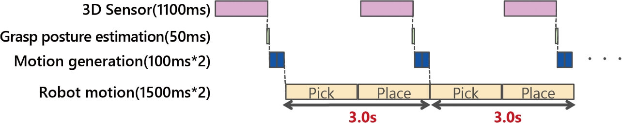
As shown in Fig. 3, the target value of 100 ms was set for a bin-picking task set as the target task.
The 3D sensor for workpiece recognition may be installed by either of the following two methods: fixed installation above randomly piled workpieces or mounting on the robot end-effector. The present study is based on the former method, which enables faster execution of the task without the need for motions for image capturing.
The bin-picking action consists of a Pick motion for picking a workpiece from a pile of randomly piled workpieces and a Place motion for placing the picked workpiece in the correct position and orientation. Assuming that a cycle time equivalent to that achievable by a human operator is set as the target, this action must be performed and completed within 3 to 4 seconds per workpiece. For the picking to be performed automatically, the Pick motion and the Place motion must be generated by selecting the workpiece to be picked and determining how to grasp the workpiece (grasp posture estimation) after the measurement and recognition of randomly piled workpieces by the 3D sensor. However, during the Pick motion, the robot comes between the pile of randomly piled workpieces and the sensor installed above, occluding the sight of the workpieces from the sensor. Therefore, the processing from measurement to Pick/Place motion generation must be fully completed within the 1.5-second duration for the Place motion. The 3D sensor for robots, up-to-date as of the development target setting, took 1,100 ms for measurement and recognition. Besides, the grasp posture estimation technology under development at OMRON back then took 50 ms for computation. Hence, the total motion generation time available for the Pick and Place motions was 350 ms. Then, based on the time required for the other overhead, including communication, the motion generation time per motion was set to 100 ms.
3. Automatic path generation technology
3.1 Related studies
Automatic path/trajectory generation technology for robots is called path/trajectory planning technology and has been the subject of many previous studies2). Classical approaches include the potential approach3) and the cell decomposition approach4). Among modern approaches are the random sampling method5-9) and approaches that handle a path/trajectory as an optimization problem10-12). In classical approaches, a robot’s passable spatial position is searched based on the real space and then converted into a corresponding robot path. Besides the high computational cost for search and conversion processing, these approaches are problematic in generating discontinuous solutions not executable because of the non-linearity between the real and joint spaces. Though low in computational cost and advantageous in that it theoretically always generates a solution, the random sampling method has the drawback of considerable variability in computational time and generated path depending on the given context. While it has a stable computational time and generates an optimal path for a set cost, the optimization approach takes a longer computational time than the random sampling method and may fail in path generation.
3.2 Evaluation and problem analysis of existing technologies
Approaches classified as a random sampling method seemed promising because of their
low computational cost and high probability of successful path generation. This subsection
explains the random sampling method, taking as an example the rapidly exploring random
trees (RRT) algorithm known as the most basic algorithm5). The RRT algorithm performs a search by growing a tree from an initial posture  toward a goal posture
  , as shown in Fig. 4:
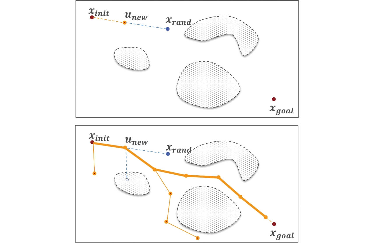
Because this algorithm performs the search in the joint space, each node in the figure represents a vector corresponding to a posture taken by the robot. In a vertically articulated robot with six joints, the joint space and the vectors are six-dimensional. The search is performed according to the following steps:
- 1. Perform sampling to pick a random node
 and find its neighbor node
  on the existing tree. The upper pane of Fig. 4 shows the results of the initial search,
where =.
on the existing tree. The upper pane of Fig. 4 shows the results of the initial search,
where =. - 2. Next, set a new node
 at a certain distance traveled from to .
 - 3. If no collision with any obstacle occurs between and , add the node and a branch connecting and to the tree.
Although the sampling method and the tree growth method may vary by algorithm, the basic processing principle is commonly shared.
From among the previous studies’ algorithms, well-evaluated ones were selected and evaluated. Table 1 shows the algorithms selected and their outlines:
| Algorithm | Outline |
|---|---|
| RRT5) | The approach illustrated in Fig. 4.  was sampled with a probability of 5% from among the sampling points to bias the implementation
used this time for the evaluation. was sampled with a probability of 5% from among the sampling points to bias the implementation
used this time for the evaluation.
|
| RRT-Connect7) | This algorithm generates one tree from each of both and to perform the search in the other tree’s direction, thereby improving the search efficiency in obstacle-sparse areas.
|
| TRRT (Transition-based RRT)8) |
If both and are at a within-threshold distance from any obstacle, this algorithm avoids adding
to the tree to prevent any proximate obstacle from impeding the tree’s growth.
|
| BIT* (Batch Informed Trees Star)9) |
This algorithm sets a subspace containing and and only searches inside, thereby improving the search efficiency.
|
For the evaluation of each algorithm, a path was generated from the initial posture to the goal posture under the conditions in Fig. 5 to measure the computational time and the success rate.
The first to third joints of the vertically articulated robot were used to change the end-effector’s spatial position, while the fourth to sixth joints were used to change the end-effector’s orientation and tilt. In other words, the robot motion was determined almost entirely based on the first to third joints. Accordingly, three obstacles were placed in between the initial posture and the goal posture to impede the robot motion along the first joint(Fig. 5(c)), the second joint(Fig. 5(b)), and the third joint(Fig. 5(a)), respectively. If these conditions did not prevent path generation, the path planning algorithm could be regarded as robust against the obstruction of the motion along any of the first to third joints and highly versatile regarding the robot motion. As far as the bin-picking action set for the target computational time was concerned, successful avoidance of colliding with the obstacle indicated by Fig. 5(a) would make the algorithm sufficiently acceptable. We, however, set the above conditions, considering the algorithm’s versatility in application to generating motions other than those for bin-picking actions.
For our evaluation, we used a computer equipped with an Intel® Core™ i5-4310U CPU running at 2.0 GHz. Considering the inherent nature of random search, we set the upper limit of computational time to 10 seconds and measured the success rate per 100 times of path generation and the computational time per success (Table 2). As a result, all the approaches evaluated showed a high path generation success rate of 90 percent or above but considerable excess in computational time from the target value of 100 ms or below.
| Algorithm | Computational time (ms) | Success rate (%) | |
|---|---|---|---|
| Average | Max. | ||
| RRT | 826 | 2086 | 97 |
| RRT-Connect | 761 | 1629 | 99 |
| TRRT | 892 | 2047 | 94 |
| BIT* | 696 | 2115 | 100 |
For algorithm improvement, we performed a problem analysis of the random sampling method. The computational time t of the random sampling method can be expressed by Equation (2):

where
- n : The number of sampling runs until the achievement of the goal posture;
- ts : The time required for sampling point generation;
- tnn : The neighbor node search time per sampling point;
- d : The distance between the node added and its neighbor node;
- Δd : The collision detection interval; and
- tcc : The time per collision detection.
Therefore, the number of sampling runs until the achievement of the goal posture and the computational time per run must be reduced to obtain a short computational time. As shown by the experiment results in Table 2, the number of sampling runs, n, and the required sampling computational time per run were 10,000 times and 0.08 ms on average, respectively.
3.3 Improvement of the search algorithm
An analysis that we performed for the existing algorithms’ search processing revealed that the number of sampling runs n increased markedly at the inlet/outlet to/from the container or the shelf. For a simple illustration of this problem, Fig. 6 shows a 2-DOF robot’s joint space and real space. Even an aperture wide open in the real space would turn into one with a very narrow robot’s passable area in the joint space, showing the difficulty in finding by random search the path from the initial posture indicated in orange to the goal posture indicated in green. This problem is known as the bug trap problem specific to random sampling13).
Known approaches to addressing this kind of problem include methods for performing searches using real-space data. Among typical algorithms is the Exploration/Exploitation Tree (EET) algorithm, which uses a virtual sphere in the real space to perform searches and feed back the results to the joint space14). This method performs searches in directions moving away from real-space obstacles and shows high search performance for bug-trap-like inlets/outlets. For non-bug-trap-like areas, however, its performance significantly deteriorates because of the lack of clues for the search. On the other hand, among the algorithms evaluated in Table 2, the RRT-Connect algorithm shows high performance for non-bug-trap-like areas. Designed in the expectation of obstacle-sparse areas in the search range, this algorithm works on the principle of generating one tree from both the initial posture and the goal posture to perform the search in the direction of the other tree. Hence, thanks to the two trees that quickly connect to each other in an obstacle-sparse area, the RRT-Connect algorithm provides high search performance.
Then, we devised a new algorithm that uses both of these two algorithms. In other words, when it finds itself stuck in a bug trap-like condition, our new algorithm uses the EET algorithm. Otherwise, it uses the RRT-Connect algorithm for path generation. As already shown by the example in Fig. 5, a bug trap may occur between a robot end-effector and a container. Bug traps can also occur when the joint value reaches or exceeds its upper limit or when a collision occurs between a non-end-effector part and an obstacle. Accordingly, our devised algorithm checks for the causative factors of all these bug traps.
This improvement of the search algorithm led to reducing the number of sampling runs, n, to 200 times or below.
3.4 Improvement of collision detection processing
Our next aim was to reduce the sampling computation time per run. A profile analysis of the computational time found that collision detection was responsible for approximately 90 percent of the processing time. Then, we considered reducing the time required for collision detection, (d ⁄Δd )·tcc .
Collision detection is performed using a 3D simulation based on the CAD data of a robot and its surrounding obstacles. As shown by Equation (2), the method commonly used is to discretize the change in the joint angle, d, between the intermediate postures on the path by Δd and check for a collision between the robot and any obstacle for each discretized posture taken by the robot in the simulation space15). Because the distance d between the intermediate postures is constant, the number of determinations can be reduced when the discretization rate is lowered by increasing the collision detection interval Δd. However, collision risks may be overlooked. Accordingly, we devised an algorithm that performs collision detection coarsely when the robot is distant from any obstacle and finely when they are near to each other as shown in Fig. 7.
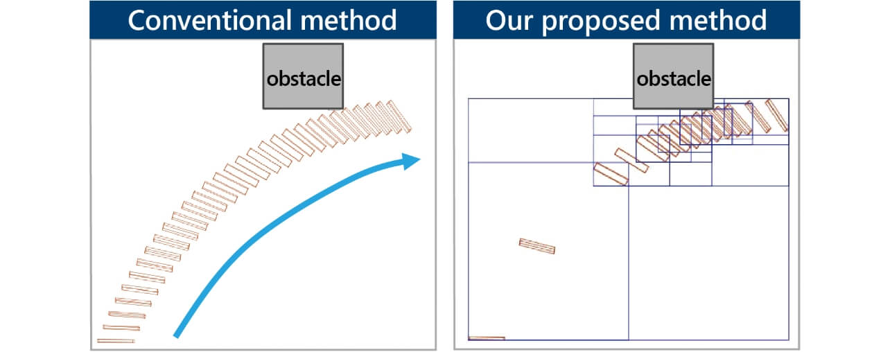
With this method, we reduced the number of determinations, d ⁄Δd, without compromising collision detection accuracy.
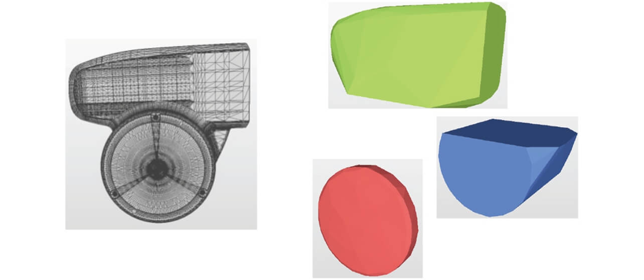
Furthermore, we aimed at reducing the computational time per run of collision detection, tcc . CAD data used for collision detection are furnished by the robot manufacturer or prepared by the user for equipment design and hence provided as high-accuracy data with many meshes ranging from several tens of thousands to several hundreds of thousands. Because the computational time per run increases in proportion to this number of meshes, desirable CAD data are those with the number of meshes reduced while retaining the geometric features. Besides, collision detection processing is known to become complicated when the model used has a concave shape. However, collision detection processing can be accelerated when the model used consists of shapes, each represented as a convex hull, and allows collision detection based on the distances between the center positions of the shapes16). Considering the above, we chose to perform collision detection processing after reducing the number of meshes in the CAD data input to the simulation space for path planning and convex-decomposing the shape model. Fig. 8 shows an example of the shape simplification of a robot’s elbow part.
We reduced the computational time per sampling run to 0.05 ms or below by incorporating the above coarse-fine search and model simplification into collision detection.
3.5 Evaluation of the automatic path generation technology
We performed an evaluation under the same conditions shown in Table 2, albeit reflecting the search algorithm and collision detection processing developed. Table 3 shows the evaluation results. The results for RRT-Connect are copied from Table 2.
| Algorithm | Computational time (ms) | Success rate (%) | |
|---|---|---|---|
| Average | Max. | ||
| Out proposed method | 28.9 | 90.4 | 100 |
| RRT-Connect | 761 | 1629 | 99 |
The above confirms that the search algorithm reduced the number of sampling runs and accelerated collision detection processing, thereby leading to the achievement of the target computational time of 100 ms.
4. Automatic motion acceleration technology
4.1 Related studies
For a robot to achieve a short motion time, it is necessary to eliminate the redundancy in the generated path and appropriately set the motion parameters. One of the technologies meeting such a requirement is trajectory planning technology, which was mentioned in reference to the related studies of automatic path generation technology. Trajectory planning technology optimizes the robot-to-obstacle distance, the end-effector’s orientation, and the torque on the joint as the parameters of the cost function, besides the robot path. Well-known technologies of this kind include Stochastic Trajectory Optimization for Motion Planning (STOMP)11) and Trajectory Optimization for Motion Planning (TrajOpt)12). The distinction of STOMP is that it performs the optimization calculation and adds random noise to the obtained results to reduce convergence to local solutions and improve the efficiency of optimum solution search. Meanwhile, what characterizes TrajOpt is that it consecutively performs convex optimization to obtain a short computational time. However, a preliminary evaluation revealed that even these efficient methods require a computational time of several seconds to several tens of seconds and are unsuitable to meet the development target of 100 ms. Besides, these methods assume the predetermination of the number of intermediate posture nodes and have the problem of being unlikely to generate a solution with too few nodes and frequently accelerating and decelerating the generated motion with too many nodes, resulting in too long a motion time.
Thus, an attempt to solve the combination of path generation/optimization and motion parameter optimization as a single optimization problem would require considerable time for the convergence of the many parameters having a tradeoff relationship with one another and would result in complicated settings. Therefore, to establish a fast optimization technology for motion parameters, we adopted a procedure that first optimizes the motion parameters based on a path generated using our path generation technology and then corrects the regions likely to affect the motion speed negatively.
4.2 Motion parameter optimization
For a robot to perform a fast motion, the two parameters of velocity and acceleration  must be maximized within a range not exceeding the robot’s torque limit. This adjustment is usually performed by tuning the velocity parameter
with the acceleration fixed. The torque on the robot’s joint is expressed by the sum of inertia torque M () and friction torque F () as shown by Equation (1). However, in a vertically articulated robot with a high
motion speed, inertia torque has the most significant influence. As Equation (1) shows,
inertia torque depends on the magnitude of acceleration, while friction torque depends
on the magnitude of velocity. It follows then that the torque load on the vertically
articulated robot’s joint becomes the largest in the timing that acceleration or deceleration was generated,
as shown in Fig. 9:
must be maximized within a range not exceeding the robot’s torque limit. This adjustment is usually performed by tuning the velocity parameter
with the acceleration fixed. The torque on the robot’s joint is expressed by the sum of inertia torque M () and friction torque F () as shown by Equation (1). However, in a vertically articulated robot with a high
motion speed, inertia torque has the most significant influence. As Equation (1) shows,
inertia torque depends on the magnitude of acceleration, while friction torque depends
on the magnitude of velocity. It follows then that the torque load on the vertically
articulated robot’s joint becomes the largest in the timing that acceleration or deceleration was generated,
as shown in Fig. 9:
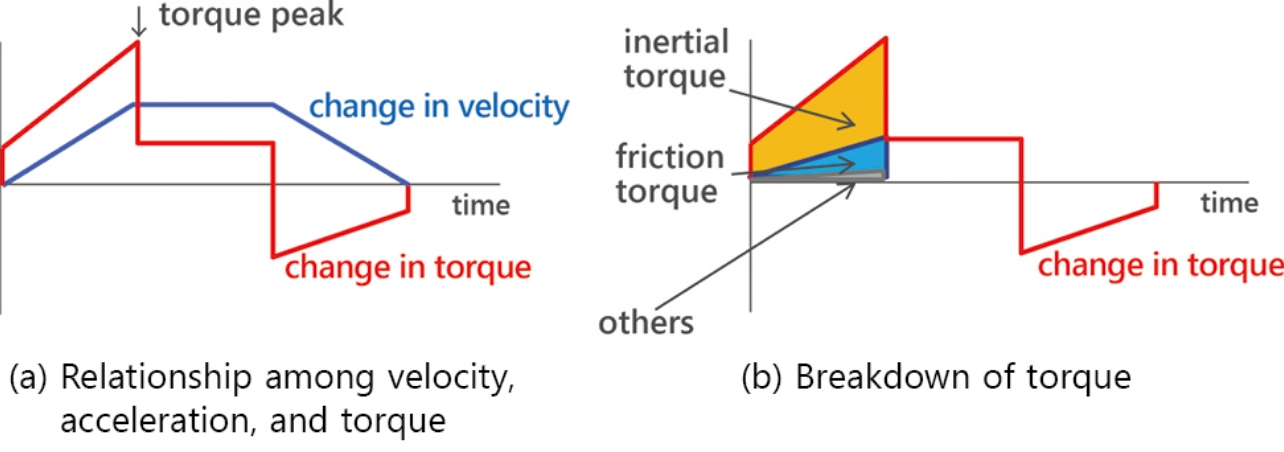
The above shows that contrary to the common practice, acceleration adjustment is more effective than velocity adjustment. Thus, we chose to accelerate the robot motion by adjusting the robot’s acceleration with its velocity fixed to either a user-specified desired value or its maximum specification value.
Acceleration adjustments are made according to the following steps:
- 1. For each joint, using a path, a given maximum velocity, and the 50 percent value of the robot’s spec acceleration, generate a trajectory and discretize it millisecond by millisecond to calculate the torque on the joint.
- 2. From the time series data of the calculated joint torques, identify the peak for each joint. If for each joint, the difference between the torque and the torque limit at the peak position is within the threshold, and if no joint exceeds the torque limit, set their accelerations as the optimal values.
- 3. If, for each joint, the peak torque exceeds the torque limit or their difference exceeds the threshold, adjust the acceleration until obtaining a value meeting the condition by binary search. Return to Step 1.
4.3 Path correction
Assuming that the robot motion is accelerated using the acceleration parameter, the
acceleration cannot be set sufficiently high if the M () term of the inertia torque M () has a large value. An M () term with a large value means that the path has on it a posture in which the joint
rotation center-to-mass point distance r shown in Fig. 10 becomes long and causes the inertia to become significant.
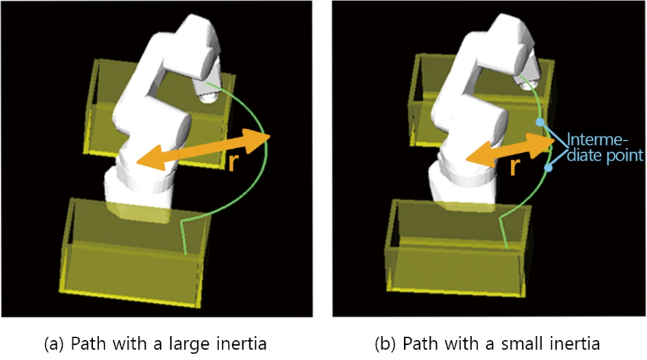
When the path is such that it causes large inertia, the acceleration can be further increased if the robot’s posture can be corrected to obtain small inertia within a range where the original motion time will not be exceeded. However, an evaluation of whether changes can be made to all the path intervals and all the joints would be a process similar to the optimization problem-solving method mentioned in reference to the related studies, resulting in a long computational time.
Accordingly, we have chosen to limit the search range focusing on each joint’s first joint and limit the path-change regions to along the joint’s second and third joints to identify regions correctable in a short time. The reason for focusing on the first joint is that the effect of reducing the inertia on an joint increases proportionally to the joint’s proximity to the root of a vertically articulated robot. Meanwhile, the reason for limiting changes to along the second and third joints is that the inertia on the first joint is attributable for the most part to the influence of the second and third joints. The correction method is as explained below:
- 1. First, from along the path, identify a continuous interval rate-controlled to the first joint as the interval to be corrected.
- 2. Based on the trajectory data, identify from the identified interval an area where the amount of change in the first joint is sufficiently large and that no motion deceleration occurs even after the intermediate points for folding the arm are added by moving the second and third joints to the interval center.
- 3. Finally, set the amount of change in the second and third joints so that the time required to undo the folded second and third joints will not exceed the time required for the first joint to move through the corrected interval.
With the above method, the path can be corrected to obtain small inertia. By the interval rate-controlled to the first joint, we mean the interval in which, among the amounts of time required for the changes made to the respective joints between neighboring intermediate points on the path, the amount of time for the first joint is the largest.
4.4 Effects of accelerated robot motion
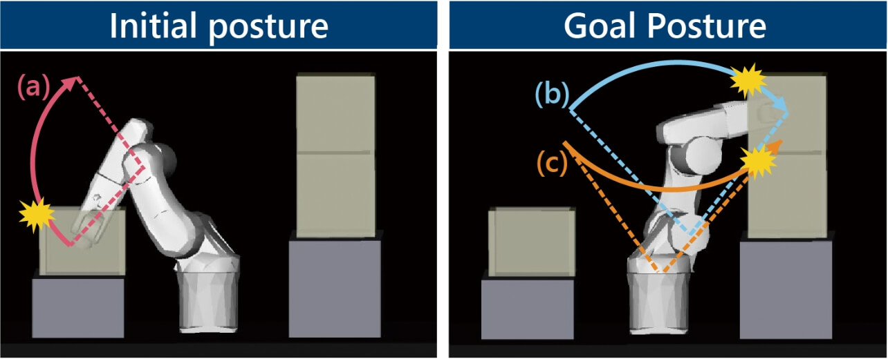
A robot’s motion speed can be boosted up to the limit using an alternating cycle of acceleration maximization through motion parameter optimization and inertia minimization through path correction. What follows in this subsection shows the results of the evaluation we performed. The experiment cases were the five patterns of motion shown in Fig. 11, in which the robot’s end-effector exited one container and entered another during a 180° movement of the robot’s first joint. A comparison was made of the motion times before and after the application of the motion acceleration technology.
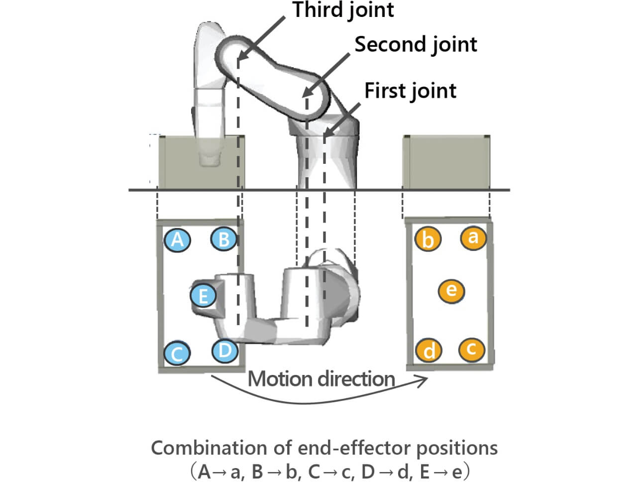
The motion times before and after the technology’s application were compared as follows to minimize the influence of the variation in the actual robot motion: the motion was performed 1,000 times before and after the technology’s application, respectively; for each run, the motion time was measured; the motion time before the technology’s application was evaluated by the minimum value in the results from the 1,000 runs; the motion time after the technology’ application was evaluated similarly but by the maximum value. For path calculation and motion optimization calculation, we used the same computer as used to evaluate the existing path planning algorithms. Table 4 shows the motion-time improvement ratio and the computational time, including path planning.
| Experiment case | Motion-time improvement ratio (%) | Maximum computational time (ms) |
|---|---|---|
| A→a | 24.7 | 95.1 |
| B→b | 19.4 | 97.1 |
| C→c | 28.1 | 96.5 |
| D→d | 28.3 | 85.3 |
| E→e | 23.3 | 90.0 |
The above confirms that a motion-time improvement ratio of approximately 20 percent was achieved with a computational time of 100 ms or below.
5. Demonstration system implemented
5.1 System overview
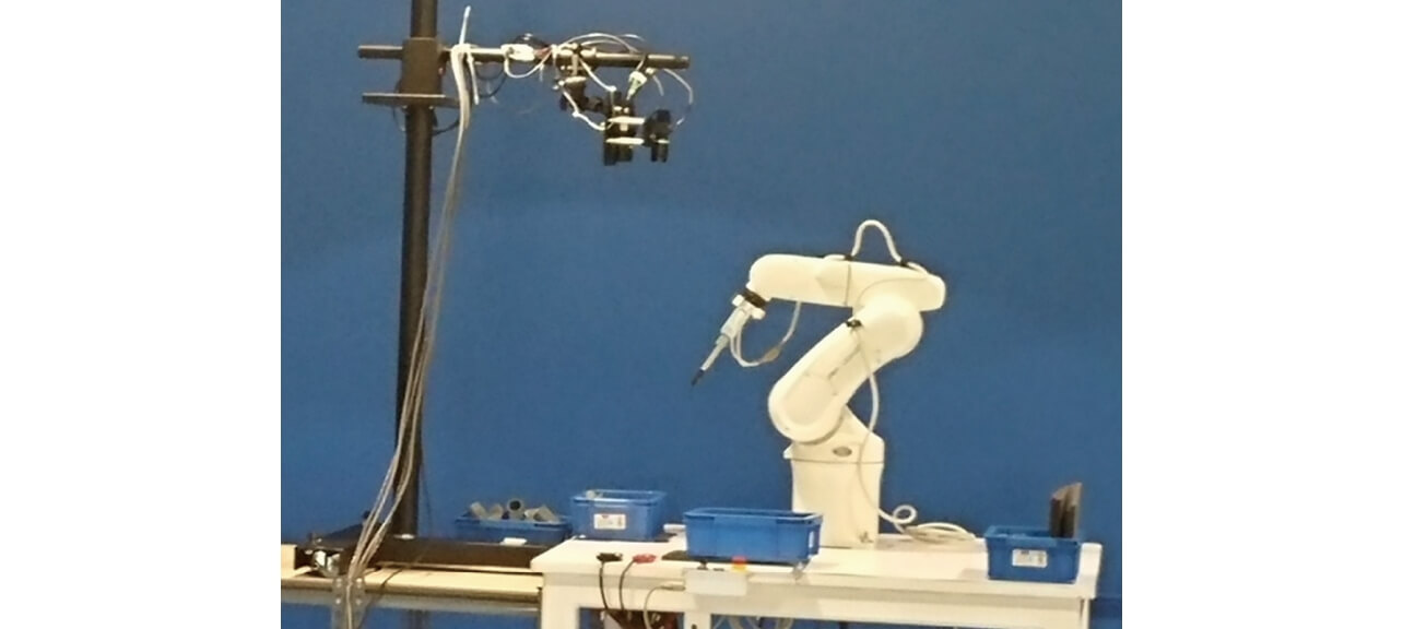
We combined the automatic robot motion generation technology developed for the present study with a 3D sensor to develop a bin-picking demonstration system. The robot used was OMRON’s Viper 650, while the sensor used for recognition processing was the robot-mountable 3D sensor earlier used for development target estimation. Fig. 12 shows the external appearance of the demonstration system.
The demonstration system served the bin-picking application without needing prior teaching or parameter adjustment except registering a prescribed set of data via the GUI. The data required to be registered were as follows:
- Sensor position
- Position of the tray containing randomly piled workpieces
- Position of the tray for aligned placement of workpieces
- Coordinates data for aligned placement of workpieces
- CAD shape of the workpiece to be picked
- Robot hand’s shape and specifications
These data are only those necessary for the equipment design. No special data are required for robot motion generation.
5.2 Performance evaluation
We evaluated the takt times achieved by the demonstration system when it performed bin picking of the six types of electronic parts. These takt times were each obtained by averaging 20 measurements of time that the system took to perform the Pick and Place motions pair shown in Fig. 3. The time from sensing to motion generation during the initial run was excluded from the evaluation. Table 5 shows the evaluation results.
| Workpiece (dimensions in cm) | Takt time (s) |
|---|---|
| A (2×3×1) | 2.9 |
| B (3×3×2) | 2.7 |
| C (15×1×0.5) | 2.9 |
| D (1×1×1) | 2.9 |
| E (1×0.5×1) | 2.9 |
| F (1×1×0.5) | 3.0 |
These results were achieved with all the required steps, from sensing to motion generation, completing within the Place motion’s duration and without the robot stopped for computational processing purposes. The above confirms that the demonstration system successfully performed the picking task at a takt time equivalent to that achievable by a human operator.
6. Conclusions
We addressed solving the problem of the difficulty in motion generation for vertically articulated robots, one of the introductory impediments of robots into production sites. We have developed an automatic robot motion generation technology that automates the position-posture setting and motion parameter adjustment tasks for robots. The automation of the former task enabled context-specific algorithm selection and efficient collision detection processing, resulting in the ability to perform motion generation in a shorter time. The latter’s automation has produced the ability to maximize the robot motion speed through the repetitive cycle of acceleration parameter optimization, highly effective on the robot’s motion time, and path correction for inertia reduction. These automation technologies are compatible with high-speed processing and hence applicable to the bin picking that requires much teaching. The bin-picking demonstration system built this time achieved a takt time equivalent to that achievable by a human operator. The development results obtained will be commercialized as bin-picking applications or robot teaching tools.
For the future, we are considering an upgrade to the automatic generation of simultaneous and collaborative motions among multiple robots to support more complex robot systems.
Acknowledgment
The outcomes of this paper were achieved through research and development from 2016 to 2019. In addition to the authors, we would like to express our cordial appreciation to Ms. NAKASHIMA Akane, Mr. MORIYA Toshihiro, Mr. TONOGAI Norikazu, Mr. SUZUMURA Akihiro, and Mr. KURATANI Ryoichi. We would also like to thank the members of the OMRON Research Center of America and OMRON Robotics and Safety Technologies, Inc., for defining the requirements and validating the commercialization of this research.
References
- 1)
- METI Kinki Bureau of Economy, Trade and Industry, “2015 Investigation of the Introductory Impediments to the Deployment of Industrial Robots to New Fields” (in Japanese), Ministry of Economy, Trade and Industry, May 31, 2016, https://www.kansai.meti.go.jp/3jisedai/report/report2015.html, (accessed Nov. 16, 2020).
- 2)
- H. Hirukawa, “Path planning problem - Robot motion planning,” (in Japanese), J. Inf. Process., vol. 35, no. 8, pp. 751-760, 1994.
- 3)
- L. A. Loeff, “Algorithm for Computer Guidance of a Manipulator in Between Obstacles,” Diss., Oklahoma State Univ., 1973.
- 4)
- J. T. Schwartz and M. Sharir, “On the ‘piano movers’ problem. II. General techniques for computing topological properties of real algebraic manifolds,” Adv. Appl. Math., vol. 4, no. 3, pp. 298-351, 1983.
- 5)
- S. M. LaValle. “Rapidly-exploring random trees: A new tool for path planning,” Dept. Comput. Sci. Iowa State Univ., Tech. Rep. TR98-11, 1998.
- 6)
- S. M. LaValle, J. H. Yakey, and L. E. Kavraki, “A probabilistic roadmap approach for systems with closed kinematic chains,” in Proc. 1999 IEEE Int. Conf. Robotics and Automation (Cat. No. 99CH36288C), 1999, vol. 3, pp. 1671-1676.
- 7)
- J. J. Kuffner and S. M. LaValle, “RRT-connect: An efficient approach to single-query path planning,” in Proc. 2000 ICRA, Millennium Conf., IEEE Int. Conf. Robotics and Automation, Symp. Proc. (Cat. No. 00CH37065), IEEE, 2000, pp. 995-1001.
- 8)
- L. Jaillet, J. Cortés, and T. Siméon, “Transition-based RRT for path planning in continuous cost spaces,” 2008 IEEE/RSJ Int. Conf. on Intelligent Robots and Systems, IEEE, 2008, pp.2145-2150.
- 9)
- J. D. Gammell, S. S. Srinivasa, and T. D. Barfoot. “Batch informed trees (BIT*): Sampling-based optimal planning via the heuristically guided search of implicit random geometric graphs,” in 2015 IEEE Int. Conf. on Robotics and Automation, IEEE, 2015, pp. 3067-3074.
- 10)
- N. Ratliff et al., “CHOMP: Gradient optimization techniques for efficient motion planning,” in 2009 IEEE Int. Conf. on Robotics and Automation, 2009, pp. 489-494.
- 11)
- M. Kalakrishnan et al., “STOMP: Stochastic trajectory optimization for motion planning,” in 2011 IEEE Int. Conf. on Robotics and Automation, IEEE, 2011, pp. 4569-4574.
- 12)
- J. Schulman, J. Ho, A. X. Lee, I. Awwal, H. Bradlow, and P. Abbeel, “Finding locally optimal, collision-free trajectories with sequential convex optimization,” Robotics: Science and Systems, vol. 9, no. 1, pp. 1-10, 2013.
- 13)
- S. M. LaValle, Planning Algorithms, Cambridge, England: Cambridge University Press, 2006, 842 p., ISBN978-0-52186-205-9.
- 14)
- M. Rickert, A. Sieverling, and O. Brock, “Balancing exploration and exploitation in sampling-based motion planning,” in IEEE Trans. Robot., 2014, vol. 30, no. 6, pp. 1305-1317.
- 15)
- C. Ericson, Real-Time Collision Detection. Florida: CRC Press, 2005, 632 p., ISBN978-1-55860-732-3.
- 16)
- A. Gaschler, Q. Fischer, and A. Knoll, “The bounding mesh algorithm,” Technische Universität München, München, Germany, Tech. Rep. TUM-I1522, 2015.
The names of products in the text may be the trademarks of each company.