














Refinement of Obstacle Constraints in Trajectory Planning Using Super Ellipses for Narrow Passage Navigation with Model Predictive Control
- Trajectory Planning
- Optimization
- Robotics
This paper presents a refinement of obstacle constraints in trajectory planning for autonomous mobile robots using Model Predictive Control (MPC). MPC generates velocity commands that guide the robot to achieve a given goal by adjusting its position and orientation over time. In MPC formulations, obstacle constraints require differentiable representations of the robot’s shape, making it difficult to directly incorporate polygonal shapes, such as squares. As a result, robots are typically approximated using primitive shapes like circles or ellipses, which introduce excessive clearance and reduce flexibility in narrow environments. To address this limitation, we adopted a shape approximation method based on super ellipses. However, high-order super ellipses often lead to instability in numerical optimization. To overcome this, we introduced a refined constraints formulation that stabilizes the optimization process. The effectiveness of this method is evaluated through simulations, demonstrating that it is more suitable for narrow passage navigation compared to conventional methods. Furthermore, the average processing time of the proposed method is equivalent to that of conventional methods, ensuring real-time performance.
1. Introduction
Manufacturing sites and logistics warehouses need numerous conveyance tasks that move items from specific points to other points. For instance, an electrical equipment assembly process involves the tasks of carrying parts from parts shelves to assembly cells. On such shop floors, many crews are engaged in conveyance tasks. However, the recent labor force shrinkage has led to high demand for automating these menial tasks. These needs for automated conveyance tasks have been addressed by introducing autonomous mobile robots. One challenge in expanding the usability of automated conveyance tasks is narrow-passage navigation. In factories and plants with limited free space, conveyance robots must be able to navigate passages with bends and constrictions, given the complex equipment layouts. Automated mobile robots with narrow-passage navigation capability would operate smoothly in such space-constrained environments, expanding their applicability in factories and plants and spreading rapidly.
Autonomous mobile robot navigation requires self-localization, path planning, trajectory planning, and various other technologies. This paper focuses on trajectory planning technology, which significantly affects narrow-passage navigation. Among representative trajectory planning methods for autonomous mobile robots is a method known as Model Predictive Control (MPC)1). MPC converts robot navigation into a model consisting of an objective function and constraint expressions and uses an optimization method to calculate velocity commands. The trajectory’s smoothness is a consideration in MPC computation of velocity commands in the prediction period. However, this method has often been avoided because of its high computational complexity. Recent improvements in computational resources implemented on autonomous mobile robots have led to an increase in studies using MPC2-5).
Generally, MPC struggles to approximate robot shapes using such polygonal primitives as squares. It struggles to formulate direct constraints against collisions with obstacles. The problem is that optimization methods used in MPC require gradients for the constraint expressions, which must be differentiable. Therefore, robot shapes are approximated with circles or ellipses for inclusion into constraint expressions. However, a simple approximation of a robot shape, such as a circumcircle, would add excess clearance around its actual contour, which would be inconvenient for narrow-passage navigation applications. Excess clearances could be reduced using a multiple-circle approach. However, additional circles pose the problem of increased computational complexity. An alternative may be an approximation method that uses a special type of superellipse, in other words, a higher-order circle (super circle), taking advantage of the property of circles that makes them increasingly closer to squares as the order increases. However, raising the order of approximation destabilizes the numerical optimization process. This paper proposes improving the constraint expression intended to address instability in the numerical optimization process that arises when using a super circle. The aim is to reduce excess clearances arising from approximation while avoiding increasing computational complexity. Our proposed method addresses the tradeoff between accurate geometric representation and computational complexity. This approach supports real-time processing and is suitable for robot navigation through narrow passages.
2. Related studies
This section overviews three well-known MPC approaches for handling robot shapes represented as polygons, such as squares.
2.1 Primitive-shape approach
The primitive-shape approach approximates robot shapes with such primitives as circles or ellipses and specifies them as constraint expressions for collision avoidance. For instance, a rectangular robot shape is often approximated using a combination of two circles2,3). The merits of this approximation are the simplicity of representations and a low computational complexity. The demerit is that approximating a rectangle with multiple primitives results in an excess clearance around it, which is inconvenient for narrow-passage navigation applications.
2.2 Mixed-integer optimization-based approach
The mixed-integer optimization-based approach6,7) combines two variables, one continuous and the other an integer, to obtain the velocity command. This approach represents a robot’s contour as a straight line, represents the left and right sides of the contour as integer values, and uses their combination to determine the inside and outside of the robot shape. Then, the robot’s trajectory is optimized to prevent the inner part of the approximated robot shape from colliding with walls or nearby obstacles. This approach has the advantage of representing a robot shape as a straight line without adding any excess clearance. On the other hand, its disadvantage is that the number of optimization combinations increases with the number of obstacles or the complexity of the passage, leading to longer calculation times and making real-time processing difficult.
2.3 Duality-based approach
The duality-based approach handles the primal problem (of finding the minimum distance between two convex sets (robot shape and obstacle convex sets)) and its dual. This approach solves an ordinary MPC model for control input calculation simultaneously with another model that finds the minimum point-to-point distance between the robot’s and the obstacle’s contours4). When a robot shape or an obstacle shape is a polygonal shape, neither is differentiable, and its model cannot be solved by the gradient method. However, converting the model into a dual problem makes the dual variable differentiable. This approach can represent a robot shape without approximation (and hence excess clearance) by solving a combination of an ordinary MPC model and its dual problem. However, it has the drawback of high computational complexity due to an increased number of variables to be solved. A more recent method reduces this drawback using a Control Barrier Function (CBF)5). However, even this method still has the problem of high computational complexity. In addition, this alternative involves a preprocessing step that approximates obstacles as polygonal shapes. When faced with a differently shaped obstacle, the method must redo preprocessing, which increases computational complexity accordingly.
3. Our proposed method
3.1 Model predictive control
Our proposed method is an improvement of the primitive-shape approach referred to as a related study in Subsection 2.12). Before describing the improvements made, this section explains the Model Predictive Control (MPC) model used as the basis. This model contains an objective function and constraint expressions.
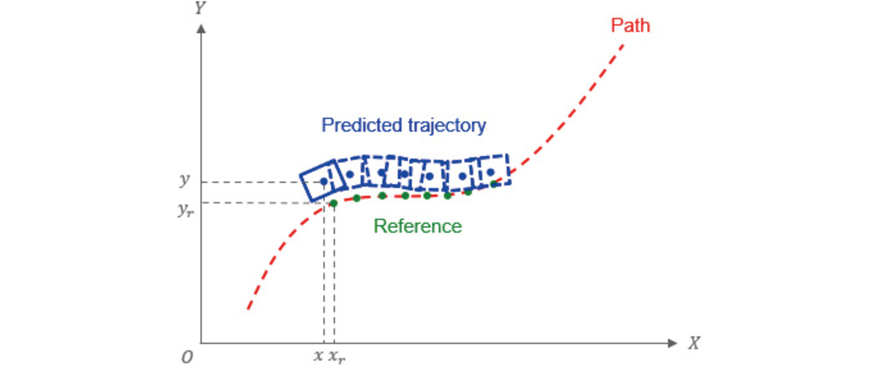
First, the objective function defines the action to be performed by the mobile robot. The action is enabled by minimizing the objective function. The objective function used in our study is represented by ϕ in (1), where x and y denote the position coordinates on the x- and y-axes in the two-dimensional plane occupied by the mobile robot, and θ denotes the rotational angle on this plane. In (1), v denotes the translational velocity, while ω denotes the angular velocity. The prediction horizon Np means that the prediction until the elapse of t seconds is performed based on the number of divisions of the time t by the time interval dt. The first and second terms on the right side of (1) denote the reference path-following terms, which indicate the difference from the reference path obtained using a method like path planning based on such information as the state of the automated guided vehicle (AGV) and the site layout. These terms are minimized to make the mobile robot travel along the reference path. Two different reference path-following terms are used: one for the terminal cost (the first term) and the other for the stage cost (the second term). The terminal cost is calculated from the difference between the AGV’s state and the reference path at the end of the prediction horizon. The stage cost is calculated from the difference between the AGV’s state and the reference path over the start-to-Np−1 interval of the prediction horizon. Fig. 1 shows a conceptual image of the reference path-following terms. Reference points (green points in the figure) are placed along the reference path to obtain a trajectory that minimizes the objective function, followed by the execution of the first-step command. This procedure is repeated to enable the robot to follow the reference path.
The third term on the right side is the input-following term, which calculates the difference between the control input and the reference velocity. This input-following term is specified, enabling easy adjustment of the moving velocity. For instance, if the robot needs to be decelerated near the goal, it suffices to specify a deceleration command as the reference velocity of this term.
The following four constraint expressions are used:
- For the kinematic constraint, we used a two-wheeled differential model identical in structure to our LD series automated conveyance mobile robot. The two-wheeled differential model is represented as (2).
- The velocity constraint is given by an inequality as in (3) and defines the upper and lower limits for the velocity achievable by the robot.
- The acceleration/deceleration constraint is given using numerical differentiation as in (4) and defines the value ranges similarly to (3).
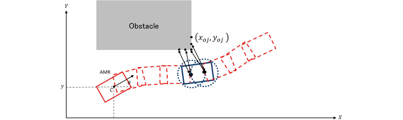
- The obstacle constraint is given as in (5) to specify a condition in which the obstacle point cloud measured by sensors is present outside the circle encompassing the robot, in other words, a condition free of collision between the obstacle and the robot. Moreover, the obstacle constraint is specified using multiple circles to encompass the robot while minimizing excess clearance. When the obstacle has no part overlapping with the red box representing the robot, as in Fig. 2, this constraint is satisfied.
3.2 Superellipse (super circle)
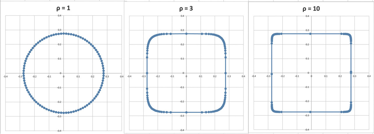
A special type of superellipse with equal major and minor axes is introduced as a super circle as in (6). As the order of (6) is raised, the circle increasingly becomes closer to a square as in Fig. 3. This property is exploited to replace a super circle for the part that specifies the obstacle constraint using multiple circles. Even when the robot has a square shape, the deviation from the actual shape can be infinitesimally reduced by increasing the order ρ of the super circle.
3.3 Super-circle-related challenge and the remedy
The challenge with using a super circle is that the value of the obstacle constraint diverges or collapses as the order increases. What is meant here by collapse is a phenomenon in which a value smaller than 1 becomes smaller and closer to 0 as the order increases. A divergence or collapse can destabilize the numerical calculation, leading to failure to solve the optimization problem. For instance, let us assume a sixth-order case with a constraint having a value of 527.2. When the order increases to 12, the constraint value becomes 527482623.1. When a value increases rapidly in this way, numerical calculations can easily become unstable. Some preceding studies8,9) use superellipses, which, however, are of low order. To address this challenge, we propose transforming the super-circle-based constraint (6) into (7). The points of this transformation are the following three:
- Point 1: Divide both sides of (6) by r2ρ, the super circle radius raised to the power of 2ρ, to prevent numerical collapse.
- Point 2: Add 1 to both sides to prevent the logarithmic value from turning into negative infinity.
- Point 3: Take the logarithm of both sides to prevent numerical divergence.
This transformation secures numerical stability. In (7), the transformation applies to both sides, and the magnitude relationship of the inequality remains unchanged. Hence, even after this transformation, collisions with obstacles can be determined.
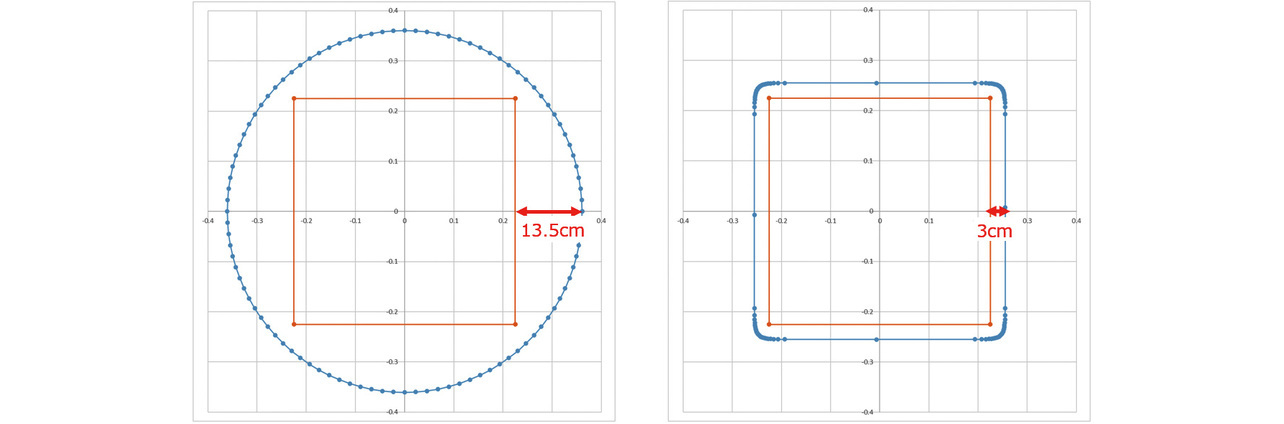
Next to be considered is the effect of using a super circle. For instance, let a square measure 45 cm on each side. Then add a 3 cm safety margin to each side to obtain a 51 cm square. Next, two versions of the obtained square are compared: one is a circle-inscribed square, and the other is a 20th-order super-circle-inscribed square. Fig. 4 shows that, when inscribed in a circumcircle, the 45 cm square has up to 13.5 cm of excess clearance around it. The excess clearance around the super-circle-inscribed square is limited to 3 cm, which is almost equal to the specified margin. Thus, when the robot shape is approximated using a super circle, its excess clearance is reduced by approximately 10 cm, enabling the robot to travel through passages 20 cm narrower than when a circumcircle is used.
Let us explain how the inequality constraint in (6) and its transformed version in (7) affect the optimization calculation to see the effect of the improved constraint expression. First, let us start with the interior point method, an optimization method. Assume an optimization problem given as (8):
where the first-line expression is an objective function, the second-line expression is an equation constraint, and the third-line expression is an inequality constraint. This optimization problem is intended to find a value of x that minimizes the objective function while satisfying the equation and inequality constraints. The Karush-Kuhn-Tucker (KKT) conditions (9) must be satisfied at an optimal point. Hence, this KKT condition is used to find the optimal value of x:
where λ and μ are Lagrange multipliers. In (9), the variables are x, λ, and μ. It is difficult to find the values of the three variables by directly solving the KKT conditions. Hence, let the KKT conditions be expanded in terms of infinitesimal variations of the variables as in (10). Here, the inequalities are ignored and replaced with 0:
The variations must be infinitesimal quantities. Hence, let a relaxation term calculated by ν, which is the mean value of (Gx−d)iμi, be added to the third equation to obtain (11):
where the scale term σ ∈ [0,1) and e is a vector consisting of components all equal to 1. When (11) is broken down into infinitesimal quantities and all the rest, (12) is obtained. The matrix that multiplies the infinitesimal quantities in (12) is called the KKT matrix.
Then, it follows that the infinitesimal quantities can be obtained by obtaining the inverse matrix of the KKT matrix and solving (13) below:
Based on the infinitesimal quantities obtained from the above, let x, λ, and μ be consecutively updated to find the optimal value of x. The constraint expressions in (6) and (7) are nonlinear constraints. Therefore, when applying (6) or (7) to the above, let its linear approximation around a point x be substituted into the expression to obtain the solution. Then, let this point be gradually updated to obtain the optimal values of the variables. The 20th-order versions of (6) and (7) linearized around and are (14) and (15). For simplicity, let it be assumed that there is only one obstacle.
Let the values of and be 2, respectively, and that of r be 1. Then, when the values of G and d are calculated for the two methods, the results will be as in Table 1 below.
| Order | Parameter | Conventional method | Proposed method |
|---|---|---|---|
| 2nd order | G | (−40, −40) | (−10, −10) |
| d | 7 | 0.653212514 | |
| 10th order | G | (−10240, −10240) | (−10, −10) |
| d | 2047 | 3.010511963 | |
| 20th order | G | (−10485760, −10485760) | (−10, −10) |
| d | 2097151 | 6.02060012 |
In the conventional method, as shown in Table 1 above, G and d showed a rapid increase in value with increasing order. With these large values, an attempt to perform the calculation in (13) fails: the values of G and Σ are too large to compute the inverse of the KKT matrix in (13), preventing the calculation of the infinitesimal quantities. Even if the initial run were successful, the infinitesimal quantities could become too large, causing updates to fail and preventing the variables from attaining optimal values. By contrast, in our proposed method, rapid increases in the values of G and d were suppressed even as the order increased. As a result, our method can stably obtain optimal solutions. These improvements are a typical effect of introducing a transformed constraint expression into the optimization method.
3.4 Formulation with the improved super-circle-based obstacle constraint
The final formulation with the improved super-circle-based obstacle constraint is (16). This problem setting used a quadratic expression as the objective function and nonlinear functions for the kinematic and obstacle constraints. Therefore, for optimization, a nonlinear optimization method was used. The nonlinear optimization method of choice in this study was Sequential Least Squares Quadratic Programming (SLSQP).
s.t.
4. Experimental evaluation
4.1 Evaluation method
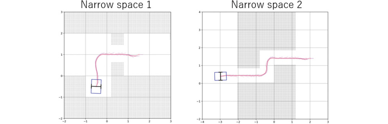
As part of the experimental evaluation to verify the effectiveness of our proposed method, we simulated to determine whether the robot could navigate narrow passages from start to goal. This experimental evaluation used a rectangular-shaped robot measuring 65 cm on the longer sides and 45 cm on the shorter sides. Two different navigation environments were prepared: Narrow Passage 1 and Narrow Passage 2. Fig. 5 shows Narrow Passages 1 and 2. Narrow Passage 1 assumed a turn for entry. Narrow Passage 2 included a crank. Each narrow passage was given two different widths: 70 cm and 80 cm.
The baseline method adopted for comparison was a multiple-circle method, which is a primitive-shape approach. The required navigation paths were calculated using a two-step application of the so-called Fast Marching Method (FMM)10). The self-localization calculations assumed ideal navigation along the paths based on the kinematic constraint expression for two-wheeled differential robots. The safety margin around the rectangular-shaped robot was set to 3 cm. The key parameters were set as follows: prediction horizon = 6; horizon time interval dt = 0.2 s; upper and lower limits for translational velocity = ±1.0 m/s; upper and lower limits for translational acceleration/deceleration = ±0.5 m/s2; upper and lower limits for turning velocity = ±180°/s; upper and lower limits for turning acceleration = ±180°/s2. The super circle was given a radius of 25.5 cm and an order n of 20. The multiple circles were given a radius of 36.1 cm to accommodate the rectangle. The evaluation metric was the processing time measured on a computer with an Intel® CoreTM i7-7700 @ 3.60 GHz CPU.
In the figure, the moving rectangle represents the robot, the gray parts represent the obstacles, and the red line represents the navigation route. The endpoint of the red line indicates the end of the navigation.
4.2 Evaluation results
As shown in the left panel of Fig. 5, Narrow Passage 1 was a case of a near right-angled entry into a narrow passage. When the narrow passage width was 80 cm as in the left panel of Fig. 6, both the multiple-circle method and our proposed method navigated the robot to the goal. With the narrow passage width changed to 70 cm, the multiple-circle method failed to solve the optimization problem in the middle, leaving the robot stranded and unable to reach the goal. On the other hand, our proposed method navigated the robot to the goal. Meanwhile, for the crank-shaped path/Narrow Passage 2 in the right panel of Fig. 5, both the multiple-circle method and our proposed method navigated the robot to the goal when the narrow passage width was 80 cm as in the right panel of Fig. 6. With the narrow passage width switched to 70 cm, the multiple-circle method ended up with the robot stranded midway. In contrast, our proposed method navigated the robot to the goal. These results show that our proposed method better suits narrow-passage navigation than the conventional method. The probable cause of the difference is that our proposed method can generate approximated robot models with smaller excess clearances and wider collision-avoidance margins against narrow passages, thereby simplifying the optimization problem.
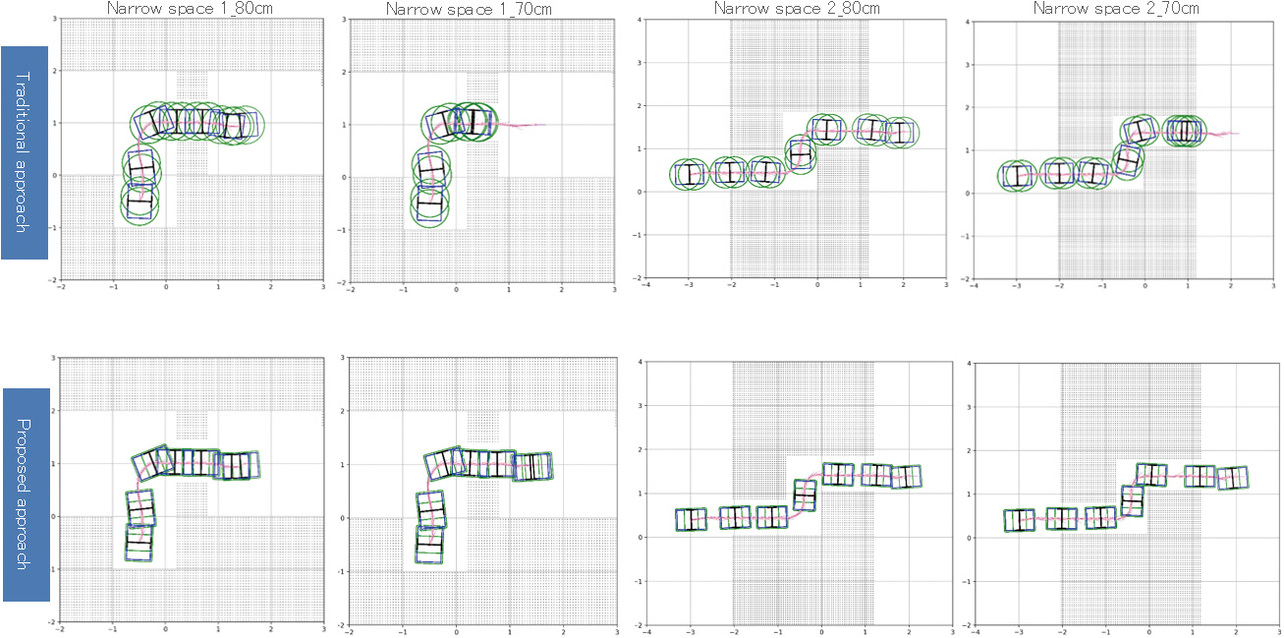
Table 2 shows the processing time results. In both methods, the optimization process was performed consecutively at each progress of the robot through the passage, with the processing time varying depending on the proximity to the obstacle. Therefore, the mean and maximum processing times were calculated for the runs of the optimization process during the robot’s navigation from start to goal for each method. The baseline method and our proposed method showed nearly no difference in mean processing time. The maximum processing time was somewhat longer in our proposed method. The likely cause was the effects of order-component calculations. Both the conventional method and our proposed method showed a maximum value of approximately 100 ms. As such, both can be said to have real-time responsiveness.
| Narrow passage | Processing time | Conventional method | Proposed method |
|---|---|---|---|
| Narrow Passage 1 80 cm |
Mean [ms] | 21 | 31 |
| Max. [ms] | 64 | 98 | |
| Narrow Passage 1 70 cm |
Mean [ms] | 53 | 29 |
| Max. [ms] | 123 | 90 | |
| Narrow Passage 2 80 cm |
Mean [ms] | 18 | 25 |
| Max. [ms] | 70 | 73 | |
| Narrow Passage 2 70 cm |
Mean [ms] | 31 | 18 |
| Max. [ms] | 110 | 118 |
5. Conclusions
This study proposes improving the obstacle constraint on the trajectory planning process of the super-circle-based MPC method for collision avoidance in robot navigation through narrow passages. The results of a comparative experiment show that our proposed method outperforms the conventional method in trajectory planning for severely conditioned narrow passages. Our method is comparable to the conventional method in terms of processing time and will serve as an effective method of robot control in applications that require real-time responsiveness.
The remaining challenges include replacing super circles back with superellipses to reduce the number of circles required and improve computational efficiency, as well as conducting operational validation with real robots. Moreover, our method is an improvement of the obstacle constraint expression and is expected to find applications in other problem settings. Examples include offline trajectory planning and path planning methods, which are among the expansions we are planning.
This study was conducted as a joint research project with Chugai Pharmaceutical Co., Ltd.
References
- 1)
- K. Felipe et al., “Model predictive control of a mobile robot using linearization,” in Proc. Mechatron. Robot., 2004, vol. 4, pp. 525-530.
- 2)
- B. Brito et al., “Model predictive contouring control for collision avoidance in unstructured dynamic environments,” IEEE Robot. Automat. Lett., vol. 4, pp. 4459-4466, 2019.
- 3)
- T. M. Cho et al., “Model predictive control of autonomous vehicles with integrated barriers using occupancy grid maps,” IEEE Robot. Automat. Lett., vol. 8, pp. 2006-2013, 2023.
- 4)
- X. Zhang et al., “Optimization-based collision avoidance,” IEEE Trans. Control Syst. Tech., vol. 29, pp. 972-983, 2021.
- 5)
- A. Thirugnanam et al., “Safety-critical control and planning for obstacle avoidance between polytopes with control barrier functions,” in ICRA, 2022, pp. 286-292.
- 6)
- A. Richards and J. P. How, “Aircraft trajectory planning with collision avoidance using mixed-integer linear programming,” in Proc. 2002 Amer. Cont. Conf., 2002, vol. 3, pp. 1936-1941.
- 7)
- L. Blackmore et al., “Chance-constrained optimal path planning with obstacles,” IEEE Trans. Robot., vol. 27, pp. 1080-1094, 2011.
- 8)
- H. Febbo et al., “Moving obstacle avoidance for large, high-speed autonomous ground vehicles,” in Amer. Cont. Conf., 2017, pp. 5568-5573.
- 9)
- P. Vlantis et al., “Quadrotor landing on an inclined platform of a moving ground vehicle,” in ICRA, 2015, pp. 2202-2207.
- 10)
- S. Garrido et al., “FM2: A real fast marching sensor-based motion planner,” Int. J. Robot. Automa., pp. 1-6, 2008.
The names of products in the text may be trademarks of each company.