


Development of Tuning Technology for Servo Driver Parameter Based on Stability Analysis and Simulation
- Control Engineering
- Gain Tuning
- Servo Driver
- Frequency Response Analysis
- Simulation
In order to meet the diversifying needs of today’s consumers, there is a growing effort to realize variable-type, variable-volume production at a cost no less than that of mass production. To this end, it is necessary to shorten the tact time and start-up time for individual manufacturing equipment. In particular, the servo drivers, which are important parts of manufacturing equipment, are expected to achieve maximum manufacturing equipment performance in a short period of time. However, most servo parameters tuning method based on time response do not quantitatively evaluate the stability of the control system. Therefore, there is a problem that the achievable performance of the manufacturing equipment, such as achievable positioning time and tracking error, cannot be fully realized, or that the control system becomes unstable from slight changes in the operating environment, such as individual differences in manufacturing equipment or workpiece changes. To address this problem, we developed an auto-tuning method for servo parameters that can bring out the maximum performance of manufacturing equipment in a short time without the need for a tuning expert by conducting a frequency analysis of the control system, including manufacturing equipment, and quantitatively evaluating the stability based on stability margins. For the stability analysis, we utilized simulation as well as actual manufacturing equipment to reduce the number of vibration tests, thereby minimizing tuning time and manufacturing equipment damage. By utilizing a simulation, about 400 combinations of servo parameters, such as notch filters, can be evaluated in a single vibration test, making it possible to realize achievable performance in a few minutes, which is difficult to reach even for tuning experts because of the limited tuning time. This method eliminates the need for on-site operators to set difficult tuning completion conditions and reduces tuning time from several days to a few minutes. As a result, customers can concentrate on building the original competence of their manufacturing equipment.
1. Introduction
Recent consumer needs have diversified. In response, vigorous efforts are underway to achieve variable-type, variable-volume production at low cost comparable to the cost of mass production as represented by the just-in-time production system. Achieving this objective requires tact time improvement and start-up time reduction in individual manufacturing equipment (hereinafter “equipment”). Servo drivers serve as an important equipment component. As such, they are especially expected to enable the equipment to achieve its maximum performance quickly. The servo driver’s built-in functions have become diversified through attempts to meet such expectations. However, our aging society with fewer children and a shrinking labor population poses a challenge in recruiting and training human resources well-versed in the servo driver’s built-in functions. Meanwhile, the current-mainstream servo-parameter tuning method is based on time-response waveforms obtained during equipment commissioning and is not intended for quantitative evaluation of control system stability. As such, this method is not problem-free. For example, it fails to extract sufficient achievable performance, including achievable positioning time or tracking error tolerance. Moreover, it allows the control system to become unstable from slight changes in the operating environment, such as the equipment’s individual differences or changes in workpieces1-4).
To address these challenges, we developed an auto-tuning method that enables even a non-tuning specialist to quantitatively evaluate the stability of a control system, including equipment, and extract the equipment’s maximum performance. This paper presents this new achievement of ours.
2. Challenges in the conventional method
2.1 Servo driver’s role and the conventional method for auto-tuning its parameters
A servo driver is device that controls the servomotor’s position and velocity to track the user-specified command value. Typical models available from us include the 1S Servo Driver Series (Fig. 1). When a servomotor is put to use, its source of electric current supply, a servo driver, requires servo parameter tuning whereby various control parameters must be optimized for the equipment. The equipment’s achievable performance or stability depends particularly heavily on the quality of feedback gain, which is used as the error correction sensitivity for the target and measured values, and that of notch filter tuning to eliminate resonance.

In servo parameter tuning, a larger feedback gain accommodates a broader frequency range (control bandwidth) for command tracking. However, excessive feedback gain leads to an insufficient phase margin/gain margin, resulting in a destabilized control system. In the conventional tuning method, the equipment’s time-response waveform is monitored to maximize the feedback gain within an equipment-vibration-free range with the aim of improving the command tracking performance. More specifically, the equipment is left to perform the operation specified for servo-parameter tuning, allowing the feedback gain to increase gradually, whereby the duration from the completion of the operation command until that of the equipment’s positioning operation remains within the target value.
2.2 Challenges in the conventional method
2.2.1 Non-conforming control architecture
Even with well-tuned feedback gain, the conventional method cannot easily obtain sufficient achievable performance if the servo driver control architecture does not conform to the purpose of the customer application.
Customer applications broadly fall into two categories, depending on their control objective. The first category includes focus-on-positioning-time applications that enable overshoot-free travel to a target position in minimum duration as in transfer applications. The second category includes focus-on-following applications that prioritize ensuring deviation-free tracking to the target trajectory as in laser cutting applications.
For positioning time reduction in a first-category application, controlling the target-trajectory acceleration/deceleration is important while expanding the feedback control system’s control bandwidth. When a user-assigned target trajectory shows considerable acceleration/deceleration, the equipment requires a proportionally large torque for acceleration/deceleration. Should the required torque exceed the servo driver’s available output range, the equipment would fall into an uncontrollable state. Therefore, positioning time reduction requires selecting a control architecture in which the target trajectory assigned to the feedback system is less likely to cause torque saturation.
For following performance enhancement in a second-category application, it is important to make corrections via feed-forward control before an error occurs. Accordingly, for a focus-on-following application, it is necessary to select the control architecture that can operate the equipment almost to the target trajectory with feed-forward torque.
Our 1S Servo Driver Series features several control architectures to meet these requirements. However, servo drivers come with diverse functions. It is impractical to expect users to spend many hours on tasks irrelevant to their primary duty just in order to understand these functions. In most cases, servo-parameter tuning is performed in the default control architecture. Hence, with a control architecture unfit for the application’s purpose, servo-parameter tuning poses the problem of failing to obtain sufficient achievable performance.
2.2.2 Insufficient level of achievable performance or stability
The conventional servo-parameter tuning method based on time-response waveforms does not allow quantitative specification or evaluation of equipment stability and, as such, is prone to either of the following problems:
- – With the target settling time being too long as the tuning completion condition, the feedback gain will fail to increase sufficiently, resulting in the inability to extract the maximum performance achievable by the equipment.
- – With the target settling time too short as the tuning completion condition, the feedback gain selected may be one immediately before the destabilization of the feedback control system. In this case, individual variations in equipment, workpiece weight changes, or other slight variations in the operating environment destabilize the control system in actual operation.
2.2.3 Equipment damage due to operating range deviation
For servo-parameter tuning based on a time-response waveform, the equipment must be operated with sufficient acceleration/deceleration before operation waveform evaluation. Its principle requires setting a large shift amount for the equipment. Accordingly, if a start point of servo-parameter tuning is near the equipment’s operating range limit, the operating range limit may be exceeded, resulting in damaged equipment. This risk adds a psychological burden to the operators responsible for servo-parameter tuning.
3. Description of our development project
This paper proposes Advanced Auto-Tuning as a tuning method that allows even a non-servo-parameter tuning specialist to extract the maximum performance from equipment quickly. This method involves no tuning completion condition parameter settings, which is too complicated for non-specialist users. Instead, it only requires the user to select the equipment’s control objective. This section consists of the following subsections:
Subsection 3.1 describes the user interface for control objective specification and explains the characteristics of the control architecture to be selected.
Subsection 3.2 explains the principle of servo-parameter tuning based on stability for extracting the equipment’s maximum performance.
Subsection 3.3 describes how to control the equipment’s operating range to within several millimeters during servo-parameter tuning and reduce equipment damage risk.
3.1 Control architecture selection through control objective specification
3.1.1 Tuning user interface
Our development project aimed to solve the problem of the control architecture selected not always meeting the control objective of the application. Hence, we developed a system that only requires the user to select and specify the control objective without needing specialist knowledge or complicated operations, such as equipment restart, for an optimal control architecture to be automatically adopted.
Fig. 2 shows a screenshot of the user interface (dialog box) for Advanced Auto-Tuning. The user should select the control objective of the application from the upper section of the dialog box and the tuning level from the three levels in the lower section. When “Focus on positioning time” is chosen from the “Control Objective” options in the upper section, the Model Following Control architecture will be selected. Alternatively, when “Focus on following” is chosen, the 100% Feed-Forward Control architecture will be selected.

Achievable performance will take precedence when the user chooses “High” from the “Tuning Level” options in the lower section. Alternatively, “Low” should be chosen to prioritize stability against changes in the operating environment.
Sub-subsections 3.1.2 and 3.1.3 describe the characteristics of the control architectures available for selection. Subsection 3.2 explains the role of the tuning levels.
3.1.2 Focus-on-positioning-time control architecture
When the control objective is positioning time, the servo driver adopts the Model Following Control architecture. Fig. 3 shows its block diagram. The Model Following Control architecture consists of a model control loop (upper section of the figure), which runs a control simulation using an equipment model, and a feedback control loop (lower section of the figure), which actually controls the equipment. Then, the equipment model’s position obtained in the model control loop is assigned as a command value (internal command value) to the feedback control loop.
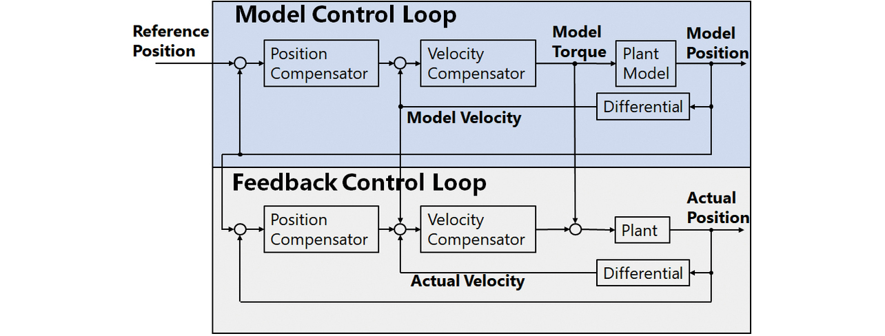
Even if the command value from the user rapidly changes, the equipment position achieved in the model control loop is assigned to the internal command value of the feedback system whereby the equipment can track the internal command value without delays. In other words, the model control loop serves as a low-path filter that eliminates frequency components that the control target cannot track from those contained in the target trajectory. This case, though deviated from the user-specified command value, translates to the target trajectory being internally generated overshoot-free during settling. The resulting settling time thus obtained is shorter than with an overshoot because of the target trajectory directly assigned to the feedback control loop.
A target trajectory is often specified by a trapezoidal velocity profile. The Model Following Control architecture likely leads to setting a high value for the maximum velocity. The responsible factor is that the model control loop functions as a low-path filter and controls the peak torque necessary for acceleration/deceleration, while acceleration/deceleration, the second-order differential of the position trajectory, is proportional to the required torque.
3.1.3 Focus-on-following control architecture
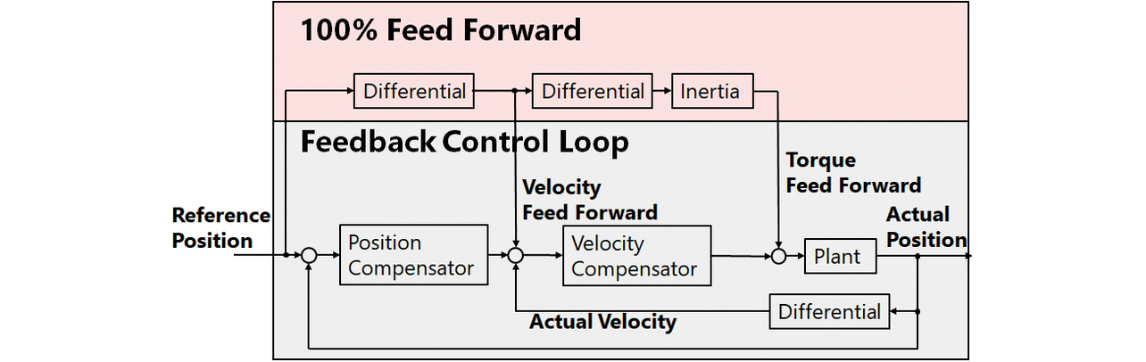
When the control objective is focus on following, the servo driver adopts a 100% feed-forward control architecture. Fig. 4 shows its block diagram. The upper section of the figure is the feed-forward section, while the lower section shows the feedback control loop. When the control target can be approximated by a single inertia, the user only has to assign the required torque calculated on the basis of the target trajectory in the feed-forward section to the control target to achieve actual equipment operation almost to the target trajectory. The feedback control loop compensates for slight errors due to the differences between the model and real equipment. If the target trajectory is free from high-frequency components that the equipment cannot track, the feed-forward control effect provides the ability to achieve high following performance.
3.2 Servo-parameter tuning based on stability
One must quantitatively analyze the equipment’s achievable performance limit and tune to extract maximum performance. Advanced Auto-Tuning uses a frequency analysis function (FFT analysis) to generate a control system stability map with feedback gain as the variable. This stability map is used to perform servo-parameter tuning in line with the application’s control objective. Sub-subsection 3.2.1 presents the specific method for this purpose.
The required number of times of real-equipment data acquisition for stability analysis should be minimized from the viewpoint of timesaving and equipment damage. Hence, after data acquisition under one specific condition, a simulation is used to reduce the number of times real-equipment data acquisition is performed. Sub-subsection 3.2.2 presents the stability map generation method using a simulation.
Besides the feedback gain, the critical parameters to be optimized to expand the control bandwidth are the number and damping characteristics of notch filters that suppress mechanical resonance. In fact, cases exist where the control bandwidth can be expanded several times through notch filter optimization. Sub-subsection 3.2.3 presents the procedure for achieving stability improvement and control bandwidth expansion through feedback-gain and notch-filter-shape optimization.
In addition to the above, Sub-subsection 3.2.4 shows the overall flow of the servo parameter auto-tuning using a stability map.
3.2.1 Principle of feedback gain tuning using a stability map
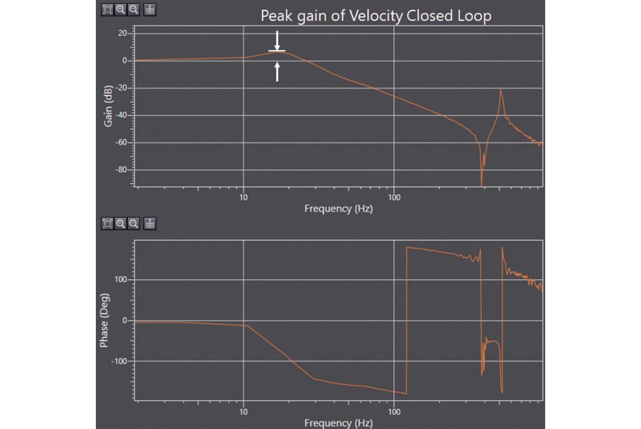
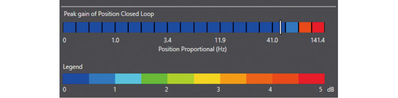
Fig. 5 shows a stability map for the velocity control loop. This figure is a contour map representing stability with the X- and Y-axes for velocity proportional gain and velocity integral gain, respectively. This stability is determined based on the FFT analysis results of an equipment vibration test performed using the representative gain of infinitesimal intervals into which the map area is divided. Fig. 6 shows the Bode diagram for the frequency transfer function of the velocity closed loop obtained by FFT analysis. The desirable gain characteristic of a velocity closed loop is that the gain remains at 0 dB until the highest achievable frequency is reached. A gain of 0 dB indicates that the equipment’s actual velocity has the same magnitude as the command velocity. A gain greater than 0 dB suggests that with the equipment’s actual velocity greater than that command velocity, the control system is becoming destabilized. The gain peak value in this Bode diagram was defined as stability with the blue stable region for 0 dB or lower and the red unstable region for 5 dB or higher.
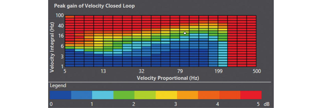
This and the following paragraphs explain how to achieve a trade-off between achievable performance and stability using a stability map. The high-frequency command tracking performance is proportional to the velocity proportional gain. Therefore, when the user-selectable tuning level is set to “High,” the largest velocity proportional gain achievable in the stable region of the stability map will be selected. For the velocity integral gain, as with the velocity proportional gain, the idea to may be to select the largest gain achievable in the stable region. However, from the viewpoint of controlling overshooting that may cause equipment wear, we set the velocity integral gain to a quarter (1/4) of the velocity proportional gain based on the coefficient diagram method5).
When the user-selectable tuning level is set to “Middle” or “Low,” feedback gain will be selected from combinations for a stability index less than 0 dB with more weight given to the stability against environmental variations. This selection translates to selecting a gain set further inside the stable region of the stability map.
As regards the position control loop gain, it is determined as follows: after the velocity-loop feedback gain is determined, a stability map with the position proportional gain as the parameter is generated to select a gain that can secure stability proportional to the tuning level similarly to the case with the velocity loop.
3.2.2 Stability map generation using a simulation
Stability map generation requires performing FFT analysis the same number of times as the number of infinitesimal intervals in the map area and then obtaining the peak gain based on the obtained Bode diagram. If FFT analysis is performed for all these infinitesimal intervals using real equipment, the data collection time and the FFT analysis time would be enormous. Moreover, the large number of vibration tests poses a risk of damage to the equipment. Hence, we used simulations for stability map generation to reduce the stability map generation time and damage to the equipment.
Fig. 7 shows the block diagram for the velocity control loop. A stability evaluation is performed based on the velocity closed-loop gain peak. As is evident from Fig. 7 regarding this point, once the equipment’s frequency transfer function is known, the other control compensation elements are also known. Therefore, the velocity closed-loop frequency transfer function can be calculated without needing a vibration test using real equipment.
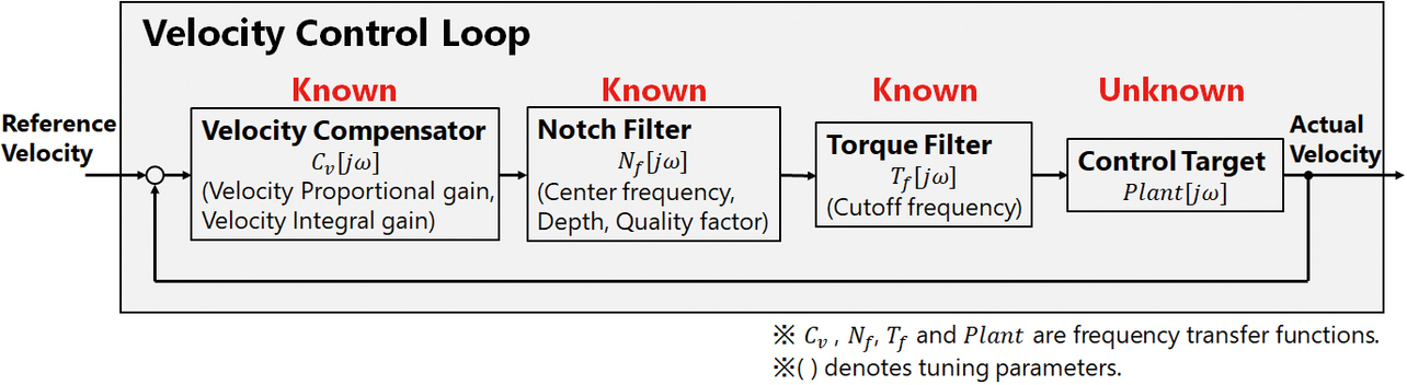
In usual practice, the frequency transfer function of the equipment is obtained by an open-loop vibration test with a torque command as the input. In contrast, in our proposed method, the control system runs a vibration test under closed-loop conditions. One reason is that performing a vibration test under open-loop conditions leads to a failure to determine the distance traveled by the equipment, which may lead to broken equipment. The other reason is to accommodate the vertical axis for the equipment falling because of feedback control failure.
Fig. 8 shows the stability map generation flow using a simulation.
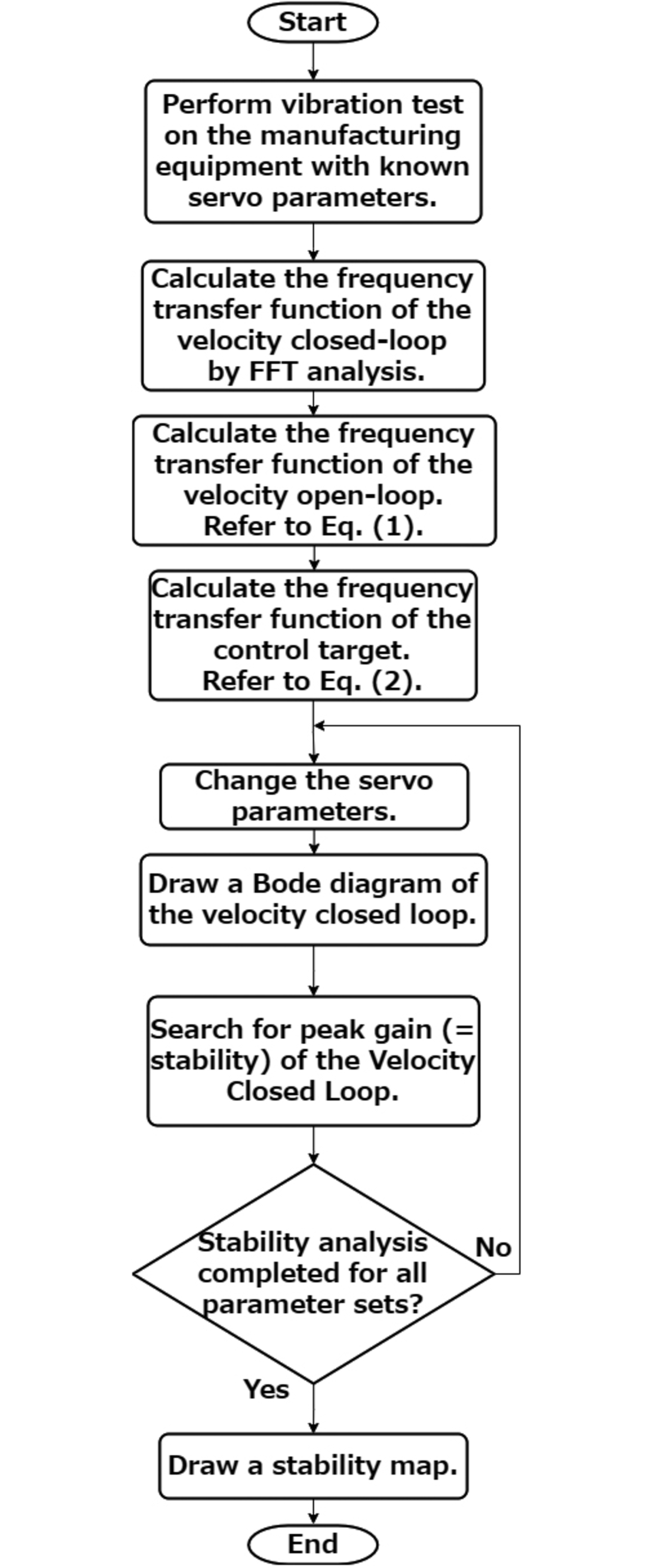
First, an equipment vibration experiment using known servo parameters is performed per the vibration pattern shown in Fig. 9. The resulting input and output waveforms are used to perform FFT analysis to obtain the Bode diagram for the velocity closed loop shown in Fig. 6. The upper section of Fig. 6 is the gain diagram. In contrast, its lower section is the phase diagram. Then, the obtained gain and phase are expressed as complex numbers to obtain the frequency transfer function (). This is used to derive the velocity open-loop frequency transfer function from Eq. (1):
Once is known, the control compensation elements are all known. Hence, the equipment-only frequency transfer function can be derived from Eq. (2), where the frequency transfer functions for the velocity compensator, notch filter, and torque filter are , , and , respectively:
Once is obtained, the above calculation is back-traced for all the infinitesimal intervals on the stability map to calculate the velocity closed-loop frequency transfer function with the feedback gain changed. The gain peak is searched from the gain diagram to generate the stability map.
3.2.3 Maximization of the stable region
Sub-subsection 3.2.2 explained how to derive a stability map with the feedback gain changed. Moreover, the velocity-loop compensator has notch and torque filters as well. The tuned quality of these filter parameters significantly affects the size of the stable region, in other words, the velocity control bandwidth. Conventionally, servo-parameter tuning engineers used to optimize the filter parameters while visually inspecting the Bode diagram. Therefore, because of the limited tuning time, there was no guarantee of achieving satisfactory optimization results. By contrast, our proposed method uses a simulation for filter parameter optimization, thereby evaluating stability for various parameter combinations and selecting a filter parameter combination for the maximum stable region.
3.2.4 Servo parameter auto-tuning flow
Fig. 10 shows the servo parameter auto-tuning flow. The auto-tuning flow goes as follows:
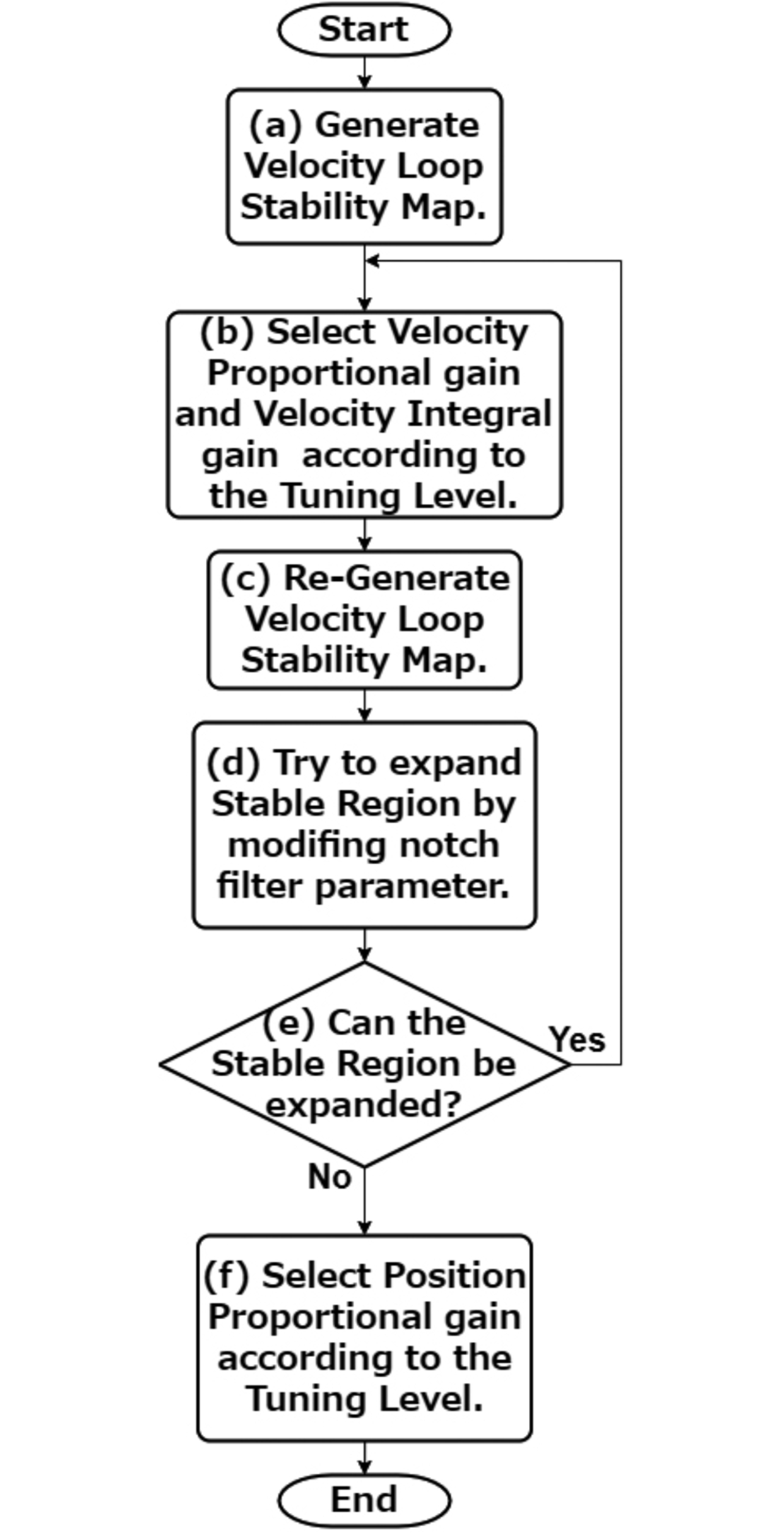
- (a)Generate a stability map using simulation based on the frequency analysis results for the velocity loop.
- (b)Tentatively determine the velocity-loop feedback gain according to the user-specified tuning level.
- (c)Using the feedback gain tentatively determined in (b), rerun the vibration test using the real equipment to obtain a more accurate stability map.
- (d)Change the notch filter parameter (center frequency, depth, or Q value). Our proprietary algorithm is followed to search for the notch filter parameter for the maximum stable region.
- (e)If the notch filter parameter change leads to a further expanded stable region, return to (b) and retry feedback gain improvement. If the stable region shows no expansion, accept the notch filter parameter and proceed to determine the position-loop feedback gain.
- (f)Generate a position-loop stability map with the position feedback gain changed.
Fig. 11 shows the position-loop stability map. The position-loop compensator is for position proportional gains only. Hence, the resulting map is one-dimensional. Similarly to the case with the velocity loop, the user-specified tuning level is followed to achieve a trade-off between achievable performance and stability and determine an appropriate position feedback gain.
3.3 Operating range control during tuning
Our proposed method subjects the equipment to vibration to determine the servo parameter based on the frequency analysis results. The equipment is vibrated with velocity feedback control enabled. Hence, the shift amount is deterministic, and the required command value amplitude for frequency analysis is within several millimeters. As such, our proposed method poses little risk that the equipment may accidentally shift outside the operating range and become damaged.
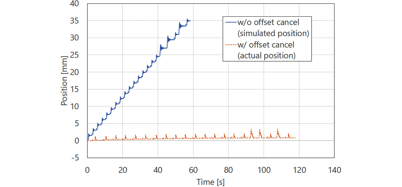
However, as shown by the servo parameter auto-tuning flow in Sub-subsection 3.2.4, the vibration operation is repeated to add more certainty to the stability map accuracy. If the equipment’s current position gradually shifts every time the vibration operation is performed, the equipment may fall outside the operating range. Fig. 12 shows with a solid line (w/o offset cancel) a typical vibration signal waveform for frequency analysis. The SweptSine waveform, which sweeps the vibration frequency over time, may end up with the final position shifted from the vibration start point (solid line in Fig. 13: w/o offset cancel).
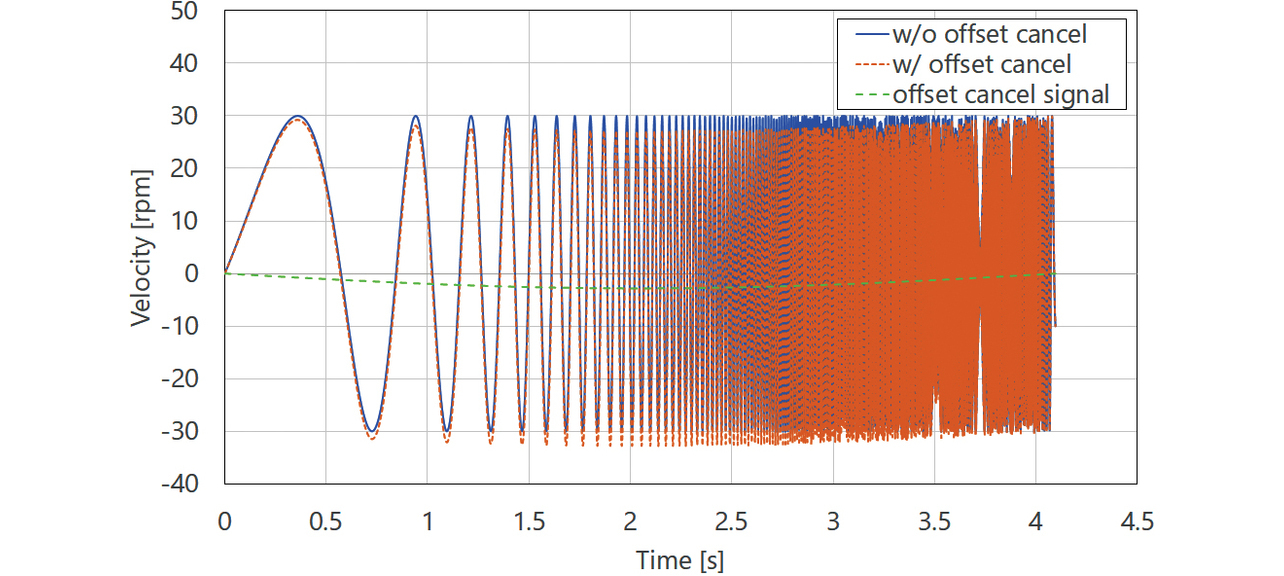
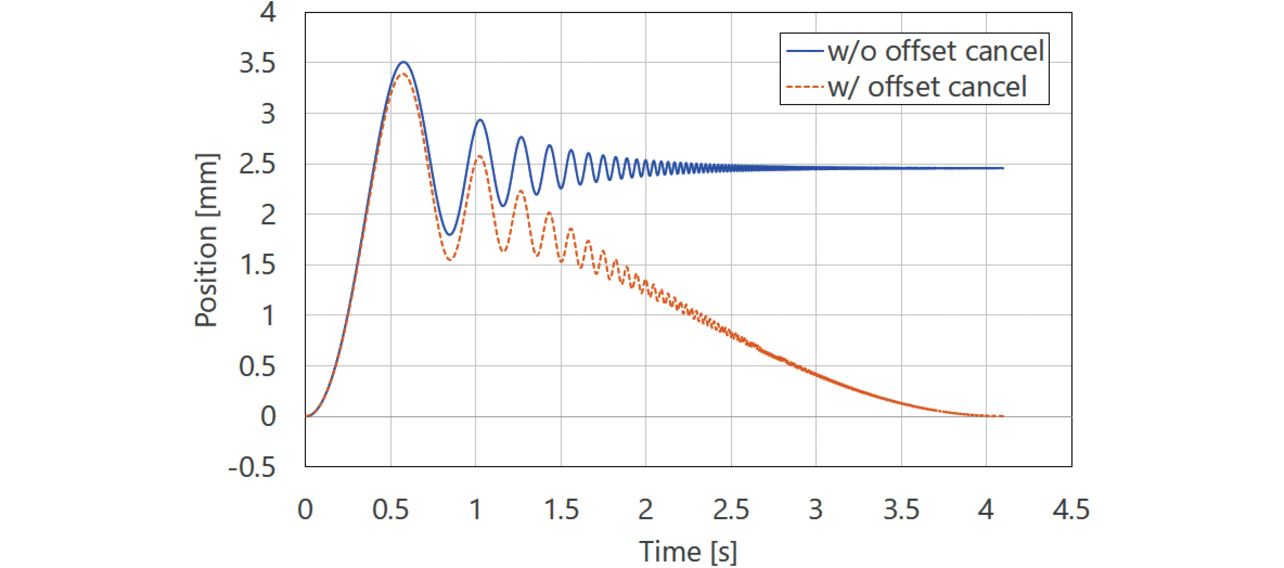
As a solution to the above issue, our proposed method provides a measure to ensure that the vibration endpoint returns to the vibration start point. More specifically, this method uses low-frequency sine wave superposition to cancel the position offset caused by the SweptSine vibration waveform. Fig. 12 shows with a dotted line (w/ offset cancel) the SweptSine waveform superposed with the low-frequency sine wave. Fig. 13 shows the position response at that point with a dotted line (w/ offset cancel).
An identification method is presented below for low-frequency sine waves to be superposed. A low-frequency sine wave to be superposed is defined as in Eq. (3), where the amplitude, angular frequency, and time are , ωL, and t, respectively:
Let the position offset caused by the SweptSine waveform before superposition be L and the total vibration time be , whereby the total shift amount of the low-frequency sine wave to be superposed is given as Eq. (4):
Complications of the identification calculation can be avoided by superposing a velocity sine wave traveling only in one direction opposite the resulting position offset. Under this condition, the half cycle of the sine wave superposed is vibration time , whereby the angular frequency ωL is given as in Eq. (5):
Substituting and rearranging Eq. (5) into Eq. (4) derives the amplitude from Eq. (6):
Substituting Eq. (5) and (6) into Eq. (3) yields Eq. (7) for the sine wave to be superposed:
4. Experiment results
4.1 Effects of control architecture selection in line with the control objective
To show the effects of adopting a control architecture in line with the control objective, we performed an experiment aiming at minimizing the positioning time and another aiming at minimizing trajectory following errors to compare the differences in achievable performance due to the difference in control architecture. The former and latter experiments used the disk load cell shown in Fig. 14 and the ball screw shown in Fig. 15, respectively. We compared two systems, one with a Model Following Control architecture (Model Following Control) and the other with a 100% Feed-Forward Control architecture (100% Feed Forward).
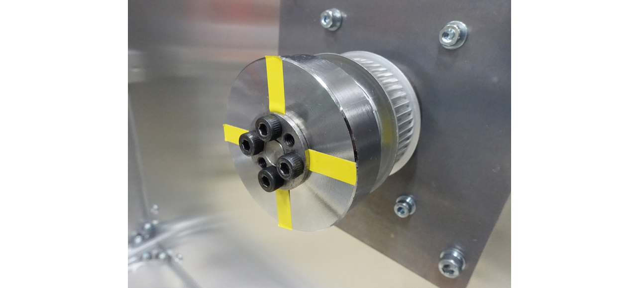
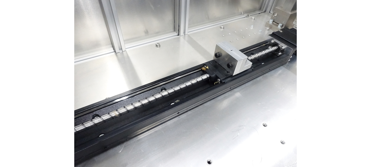
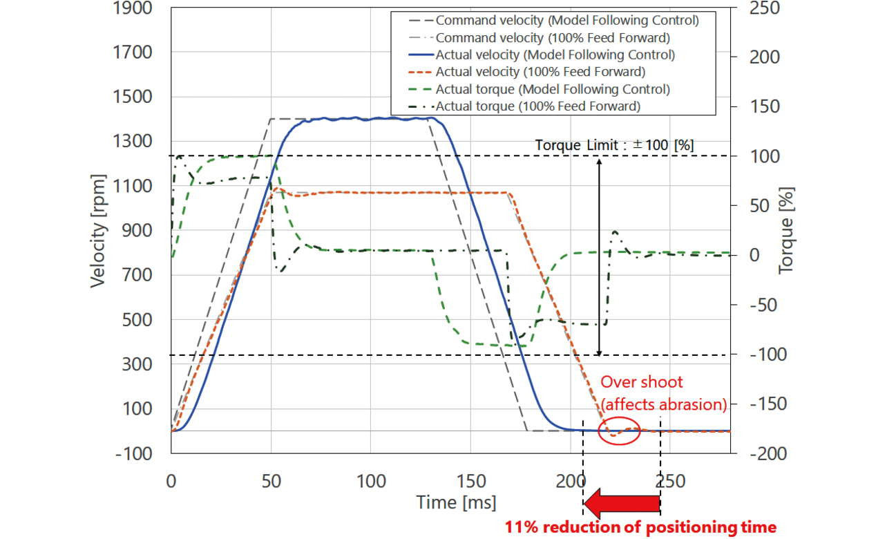
Fig. 16 shows the positioning time differences due to the difference in control architecture. For each control architecture, this figure shows a target trajectory at the maximum velocity achievable without the torque output limit being exceeded. Table 1 shows the experiment conditions. The Model Following Control architecture exhibited a discrepancy between the target trajectory and the internal command value. On the other hand, this architecture allows overshoot control, reducing damage to the equipment. It also allows torque saturation control, whereby the maximum velocity can be set high. As a result, its adoption led to positioning travel time reduction by 11% relative to the 100% Feed-Forward Control architecture.
| Condition | Value |
|---|---|
| Maximum velocity (Model Following Control) | 1070 rpm |
| Maximum velocity (100% Feed-Forward Control) | 1400 rpm |
| Acceleration/deceleration time | 50 msec |
| Distance traveled | 3 revolutions |
| Torque output limit | ±100% (± 0.318 N·m) |
| Advanced Auto-Tuning’s tuning level | Middle |
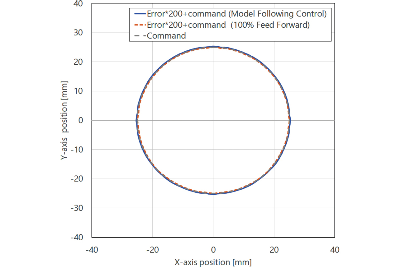
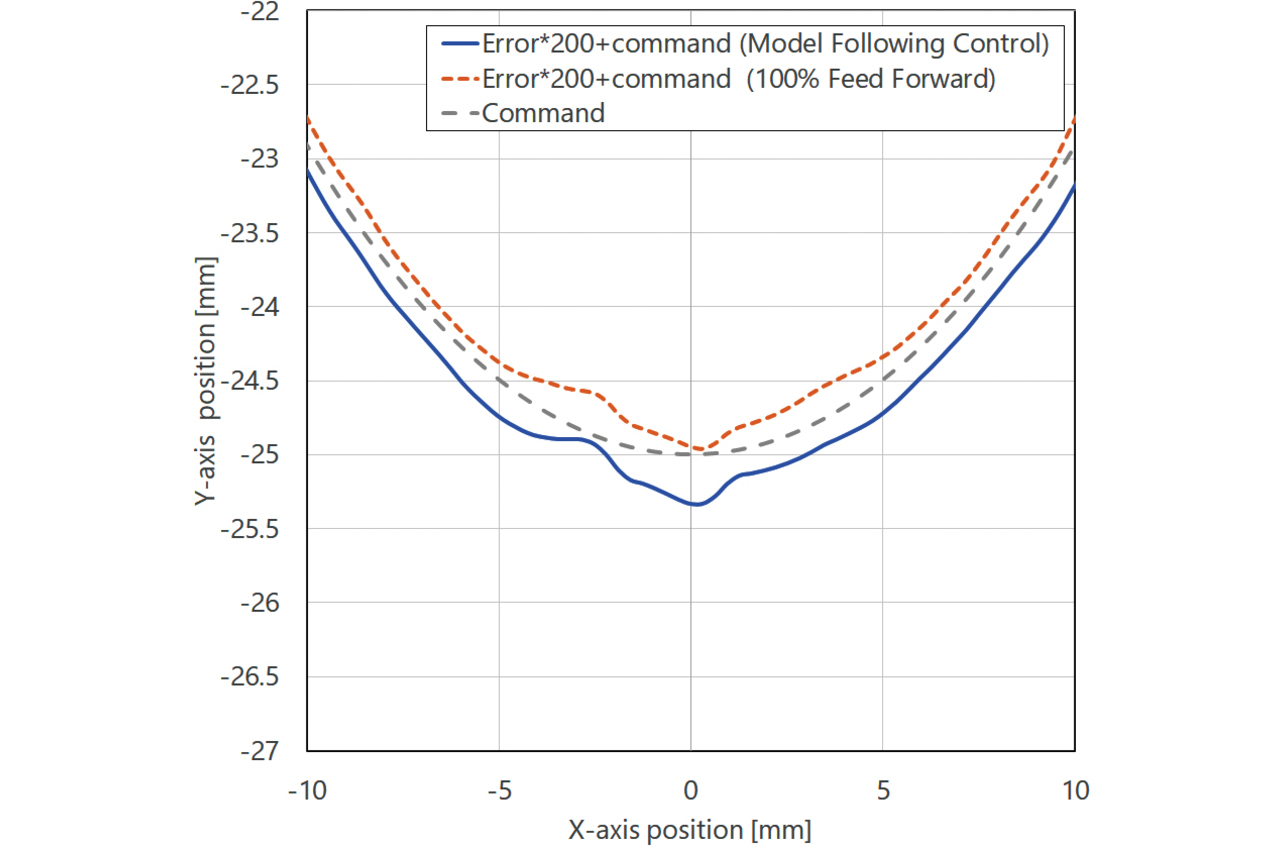
Fig. 17 shows the difference in the target trajectory following performance due to the difference in control architecture. Two hundred times magnifications of errors to the respective target trajectories are shown by the error circles added to the target trajectories. Fig. 18 is an enlarged view of the quadrant glitch in which the tracking error becomes the largest6). Table 2 lists the experiment conditions, while Table 3 shows the mean and maximum errors to the target trajectory for each control architecture. Table 3 reveals that the 100% Feed-Forward Control architecture for applying via feed-forward control the required torque estimated based on the target trajectory showed 42% lower tracking errors than its Model Following Control counterpart. These observations show that the Model Following Control architecture with a low-path filter effect to the target trajectory is unsuitable for focus-on-following-target trajectory applications.
| Condition | Value |
|---|---|
| Circle radius | 25 mm |
| Angular velocity | 2π rad/s |
| Advanced Auto-Tuning’s tuning level | Middle |
| Error to the target trajectory | Model Following Control | 100% Feed-Forward Control |
|---|---|---|
| Mean error | 1.1 μm | 0.7 μm |
| Maximum error | 4.1 μm | 2.4 μm |
4.2 Effects of stability analysis-based tuning
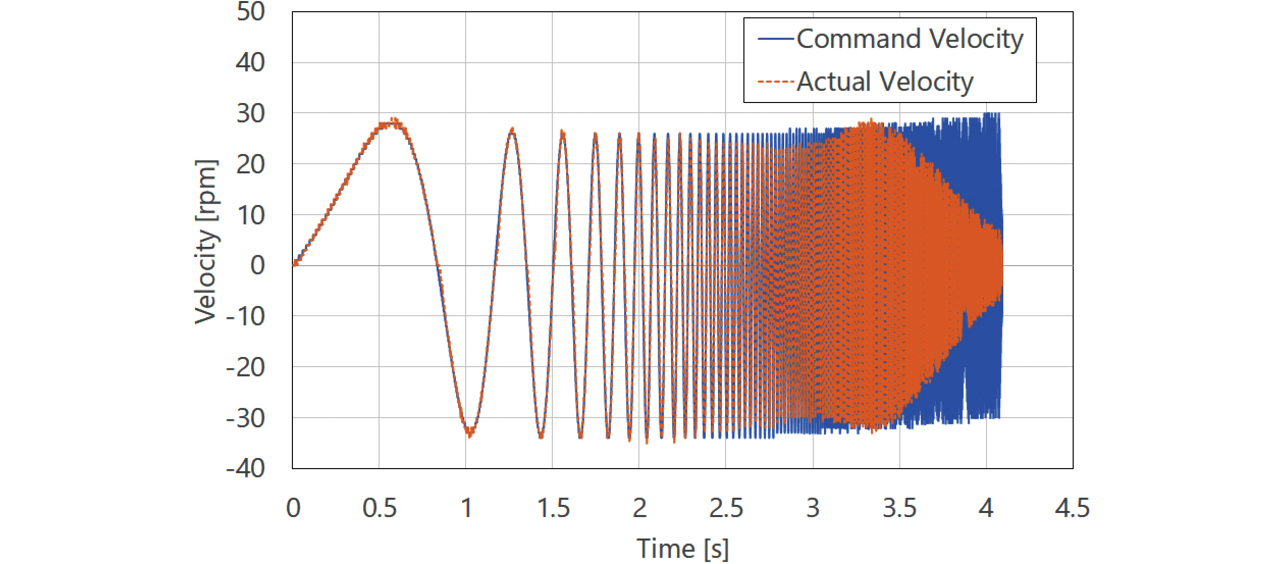
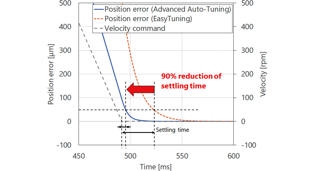
Fig. 19 shows the comparison results for settling time between the gain tuning method (Easy Tuning) based on the conventional time-response waveform and our method (Advanced Auto-Tuning). The control architecture and target settling time for Easy Tuning were set to the default values, in other words, “Model Following Control” and “50 ms,” respectively. Our method’s control objective and tuning level were set to “Focus on positioning time” and “Middle,” respectively. Table 4 shows the other experiment conditions. Both control architectures are equally a Model Following Control architecture. Our method increases the feedback gain to expand the control bandwidth while quantitatively evaluating the feedback system’s stability. As a result, it reduced the settling time by as much as 90% relative to Easy Tuning.
W/O stability analysis: Easy Tuning W/ stability analysis: Advanced Auto-Tuning
| Condition | Value |
|---|---|
| Maximum velocity | 500 rpm |
| Acceleration/deceleration time | 50 msec |
| Distance traveled | 3 revolutions |
Fig. 20 shows the comparison results (error circles) for the following performance of Easy Tuning and our method (Advanced Auto-Tuning). Our method’s control objective and tuning level were set to “Focus on following” and “Middle,” respectively. The rest of the experiment conditions are the same as shown in Table 2. Our method adopts a 100% Feed-Forward Control architecture, which involves no internal filtering of the target trajectory. Moreover, the feed-forward torque enables delay-free operation to the target position. Furthermore, our method expands the control bandwidth to the maximum while quantitatively evaluating stability, thereby enabling rapid correction of quadrant glitches not included in the equipment model. As a result, it reduced trajectory following errors by as much as 98% relative to Easy Tuning.
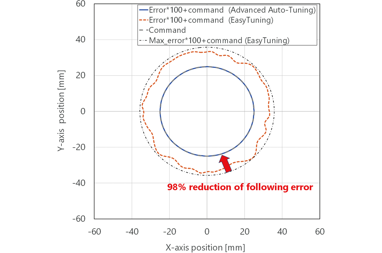
W/O stability analysis: Easy Tuning W/ stability analysis: Advanced Auto-Tuning
4.3 Effects of operating range reduction during tuning
Fig. 21 shows the superposition effect of a low-frequency sine wave canceling the position offset caused by the SweptSine vibration waveform. Our proposed method (Advanced Auto-Tuning) runs the vibration test on the equipment up to approximately 40 times by the time of tuning completion. Without our proposed method, the 10 mm lead-pitch ball screw exhibited an approximately 35 mm equipment shift by the completion of tuning. On the other hand, with our proposed method, the maximum shift amount per vibration test was reduced to 2.5 mm, while the measured position offset amount after the 39th vibration was reduced to 0.8 mm. These observations mean that our proposed method can reduce to very low levels the risk of equipment shifting outside the operating range and getting damaged, thereby helping to reduce the psychological burden on the operator.
5. Conclusions
The conventional servo-parameter tuning method based on time-response waveforms has challenges, such as being unable to obtain sufficient achievable performance or ending up with the equipment being unstable even at slight changes in the operating environment. To solve these challenges, we proposed a servo-parameter tuning method that enables even a non-servo-parameter tuning specialist to extract equipment’s maximum performance by just specifying the control objective.
Our proposed method uses frequency analysis technology to quantitatively evaluate the stability of a control system, including equipment, to achieve a trade-off between achievable performance and stability. For stability analysis, we reduced the number of equipment vibration tests using a simulation besides real equipment to reduce the tuning time and damage to the equipment. Through the use of simulation, our proposed method enabled approximately 400 patterns of evaluation per vibration operation for combinations of servo parameters, such as notch filters, thereby enabling the successful attainment of the achievable performance in a few minutes, a feat difficult for even a tuning specialist to perform because of the constraint of limited tuning time. Moreover, we creatively improved the vibration trajectory in frequency analysis to control the equipment’s operating range to within several millimeters, helping to reduce the risk of broken equipment due to incorrect operations and alleviate the psychological burden on on-site operators. As regards stability, we gave it visibility through the conversion into stability maps with a feedback gain as the variable. This visualization method enables an intuitive estimation of the achievable limit of control bandwidth or margin of stability. It will provide a promisingly useful method to help avoid continuously pursuing unachievable performance or to evaluate the degree of improvement in the mechanical rigidity of equipment.
Moving forward, we will deploy the above-described servo driver parameter tuning method using stability analysis and simulation to equipment with several mechanically connected motors to expand the range of compatible applications.
References
- 1)
- OMRON, “Control apparatus and method for tuning servomotor,” (in Japanese), Japanese Patent No. 6409886, Oct. 24, 2018.
- 2)
- OMRON, “Processing apparatus, control parameter determination method, and control parameter determination program,” (in Japanese), Japanese Patent No. 6460138, Jan. 30, 2019.
- 3)
- OMRON, “Setting support apparatus,” (in Japanese), Japanese Patent No. 7119760, Aug. 17, 2022.
- 4)
- OMRON, “Setting support apparatus,” (in Japanese), Japanese Patent No. 7119761, Aug. 17, 2022.
- 5)
- S. Manabe and Y. C. Kim, Coefficient Diagram Method for Control System Design, Springer, 2022.
- 6)
- A. Matsubara, Design and Control of Precision Positioning and Feed Drive Systems, Morikita Publishing, 2008, pp. 185-198.
The names of products in the text may be trademarks of each company.