


Improved Anomaly Detection in Data Affected by Sudden Changes in the Factory
- AI technics
- Realtime anomaly detection
- Quality control
- PLC
- Machine learning algorithm
Solving labor shortages and improving product quality are major issues at manufacturing sites, and artificial intelligence (AI) is being applied as a means of improvement. However, there are cases where it is difficult to apply conventional AI. One such case is the discrepancy between the distribution of data assumed by AI algorithms and the data at the actual manufacturing site. At the manufacturing site, there are fluctuations in many factors, such as changes in raw materials, replacement of jigs, and changes in equipment settings, and the data are affected by them. If there are such fluctuations, then any sudden fluctuations would also appear in the data.
Conventional AI assumes that there will be no sudden fluctuations. Therefore, when conventional AI is applied to cases where the influence of any fluctuations is large, it results in erroneous judgments. This improvement is one of the challenges in utilizing AI.
In this paper, we propose a new algorithm that adds the control chart method that has been conventionally used in the field of quality control to the conventional algorithm. And for on-site issues that were difficult to deal with using conventional algorithms, the false positive rate of the proposed method was 18%, while the two conventional methods were both about 70%. This algorithm can improve the false positive rate by about 50% and has been confirmed to be effective. In this paper, as an AI that can respond to fluctuations in data, we show the direction by an algorithm that combines the detection of fluctuations by the control chart method and sequential learning.
1. Introduction
The most common purpose of introducing AI is probably to reduce or replace human tasks. For instance, OMRON explains the effects of introducing AI, using such phrases as “... making active use of AI to reproduce the skills of skilled inspectors” or “... new man-machine cooperation for making a revolutionary difference to workforce productivity and quality on the shop floor of food products manufacturing.”1)
AI solutions come in various forms or with various algorithms. Particularly widely used are the so-called machine learning algorithms2). Machine learning involves the tasks of preparing data and making the machine learn them. A learned machine can make predictions or determinations and perform other operations. This functionality enables machines to replace human acts of making predictions or determinations. For example, in the case of a manufacturing site, such as mentioned above, a machine learning model is built using learning data collected from the machinery and various sensors and then is applied to detect anomalies on the manufacturing site.
Batch and sequential learning have been conventionally known as machine learning application flows3). Batch learning is a method of learning by preparing a certain amount of data as learning data and batch-processing them. After the learning phase, the AI-based prediction or determination phase follows. In batch learning, learning data collection periods mean AI downtimes. An OMRON product, an AI-equipped machine automation controller, is also of this type4).
Sequential learning is a method in which learning is repeated each time the sample size increases. In sequential learning, no batch learning is performed using new learning data in addition to past learning data every time the sample size increases. Instead, the cycle repeats itself of correcting past learning results with new samples. This cyclic process saves the need to handle large amounts of sample data simultaneously, reducing the computational complexity. Moreover, the learning and AI use periods proceed simultaneously, eliminating the need for time to accumulate learning data.
In batch learning, the learning and prediction phases are thus separated, making it impossible to track fluctuations in data distribution. In sequential learning, while fluctuations in data can be tracked, learning is easily affected by temporary fluctuations. Besides, changes in distribution are tracked slowly due to the effect of past data.
As detailed in the next section, such fluctuations may occur even with all imaginable conditions fixed, posing one of the challenges in applying machine learning to manufacturing sites. To solve this challenge, this paper proposes a new algorithm that combines fluctuation detection by the control chart approach with sequential learning. Section 2 presents the challenges to be solved in this paper, while Section 3 presents a proposed method. Section 4 shows the results of an experiment using specific equipment. Section 5 discusses the proposed method based on the experiment results.
2. Challenges
When data are continuously collected, trends may significantly change at different times. At a manufacturing site, this phenomenon can occur because of many factors, such as material changes in raw materials, replacement of jigs, and changes in equipment settings.
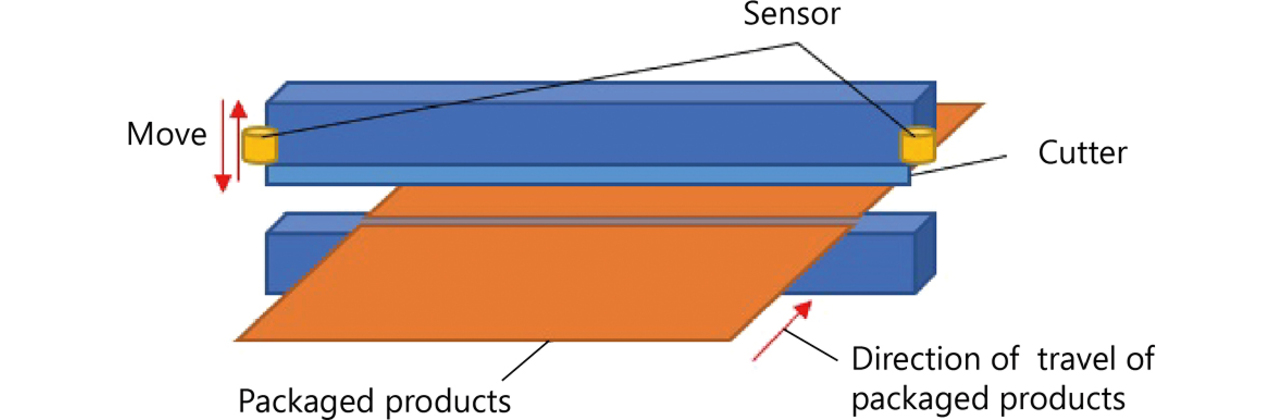
This paper explains this challenge using the cutter position data at the moment of cutting in a horizontal pillow packaging machine. A horizontal pillow packaging machine wraps to-be-packaged items with rolled film and heat-seals them into packaged products. Finally, individual packages are completed as cut off from the film. This cutting is performed using a cutter: in the experimental setup, a displacement sensor is fitted on each end of the cutter to measure the cutter height at the time of cutting performed by the cutter during its vertical motion. With two displacement sensors provided, data are collected in pairs at identical times. Fig. 1 shows a schematic view of the cutter:
Figs. 2 and 3 show the data from the respective sensors. These data are those with the packaged dimensions, the material, and the to-be-packaged item being the same, excluding data from under different conditions midway. The vertical axis in the figures indicates the measured value extracted from the actual displacement sensor data and processed by multiplication with a constant. The cutter height varies during a single cycle consisting of a sequence of actions, such as transferring and cutting the to-be-packaged item. This height is measured as displacement. From such cycles, only the values of the cutter height at the moment of cutting are extracted as data for use in this paper.
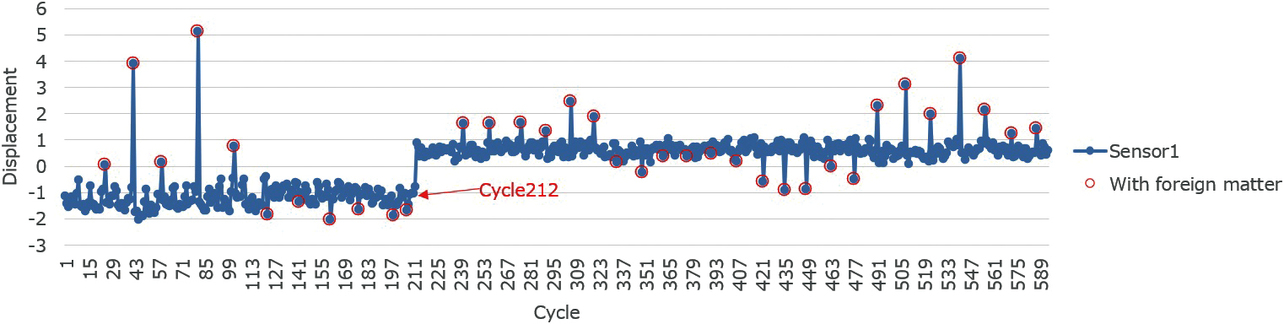
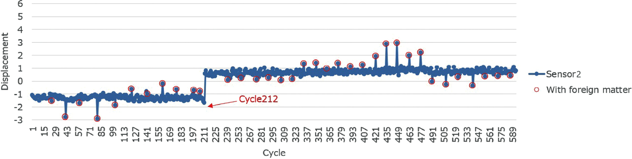
The red circles in Figs. 2 and 3 indicate when foreign matter was intentionally jammed in. With foreign matter present, outliers tended to be more pronounced than with foreign matter absent before and after. Sometimes, the Sensor 1 value outlay to the positive side, while the Sensor 2 value outlay to the negative side; at other times, the other way around. In the experiment, the experimenter selected the foreign matter position. Hence, it is a given that the orientation of outliers depended on the relative position of the foreign matter to the two sensors.
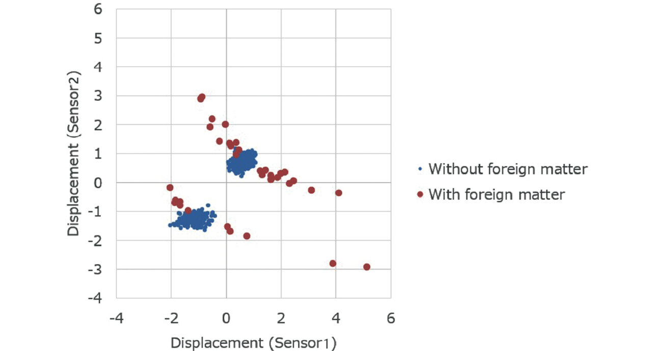
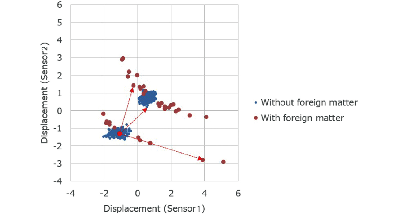
Fig. 4 shows the scatter diagram for the data from Figs. 2 and 3. Data points representing samples without foreign matter are distributed in clusters around two regions. These two regions are the areas before and after Cycle 212. Data points representing samples with foreign matter are shown distributed with features different from those of such clusters.
The AI of interest to this paper is intended to determine whether a non-defective or defective product results immediately after processing. For this purpose, the judgment is made based exclusively on the real-time processing data rather than by an inspection process placed downstream of the processing.
The challenge to be solved specifically by this AI is cases with a significant change occurring midway as in Figs. 2 and 3. We had to address these cases when developing an AI for packaging machines. The data in Figs. 2 and 3 are the records of values measured over the lapse of time. In Fig. 2, the displacement ranges between −2 and 0 until Cycle 212 but ranges between 0 and 1 after Cycle 212, indicating that a significant change occurred at that time. Fig. 3 similarly shows a significant change at the time of Cycle 212.
Fig. 5 shows the results of using the MT method5), a type of batch learning, as the conventional anomaly detection method. The samples from Cycle 1 to Cycle 24 were used as learning data sources. The vertical axis in Fig. 5 indicates the Mahalanobis distance (MD). See 3.2.1 for the explanation of the Mahalanobis distance.
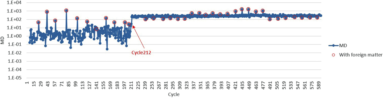
This method compared the MD values for samples with and without foreign matter until Cycle 212, revealing that samples with foreign matter showed a high MD value. Until Cycle 212, the MD values around between 1.E+02 and 1.E+03 corresponded to samples with foreign matter. The MD values after Cycle 212 lay around between 1.E+02 and 1.E+03 regardless of with or without foreign matter. For example, with a rule that samples with 1.E+01 or more are determined defective, many of the samples without foreign matter would be determined non-defective until Cycle 212. After Cycle 212, however, all the samples without foreign matter would be determined defective. Hence, the rule is unusable as a determination mechanism.
For this example, we used the MT method as the machine learning algorithm. However, the problem herein arose due to the flow of batch learning per se. Even with other machine learning algorithms, if based on batch learning, similar problems will occur.
The first challenge encountered in addressing cases such as those in Figs. 2 and 3 is how to automatically detect changes occurring after Cycle 212. Another challenge is how to start determination quickly based on a new criterion after detection. Besides, with single cycles of the packaging machine being on the order of 0.1 to 1 second, how to achieve high-speed computation with low computational complexity poses yet another challenge.
3. Proposed method
This section proposes a method that discards the current criterion upon detecting a change posing a challenge and starts learning anew. With sequential learning as its basis, this method can accommodate the challenge of high-speed computation while making it possible to start determination quickly based on a new criterion after detecting the change. This way, solutions have been achieved to the challenges presented in the preceding section.
3.1 Run-based learning flow
The first thing required to solve our challenges is a method of automatically identifying the timings of changes. We decided to apply an index called a run6) in the control chart approach as this method.
A run is an index that regards a situation as an anomaly when the value under monitoring occurs on either the positive or negative side to the central value of 0 consecutively a certain number of times. The JIS6) defines a run as nine consecutive occurrences. The probability of a situation where the value occurs on the positive side nine consecutive times is given as follows:

The idea of run assumes that when a situation with such a low probability of occurrence has occurred: something anomalous has occurred; hence, something unlikely to occur by chance has occurred but not that the event has occurred by chance.
Fig. 6 shows a flowchart for determining the occurrence of a run. The value sxn in Fig. 6 is obtained for the newly obtained data xn from the average value (Ave) and standard deviation (Std) of the data prepared before putting the flow into operation. This process is called standardization7).

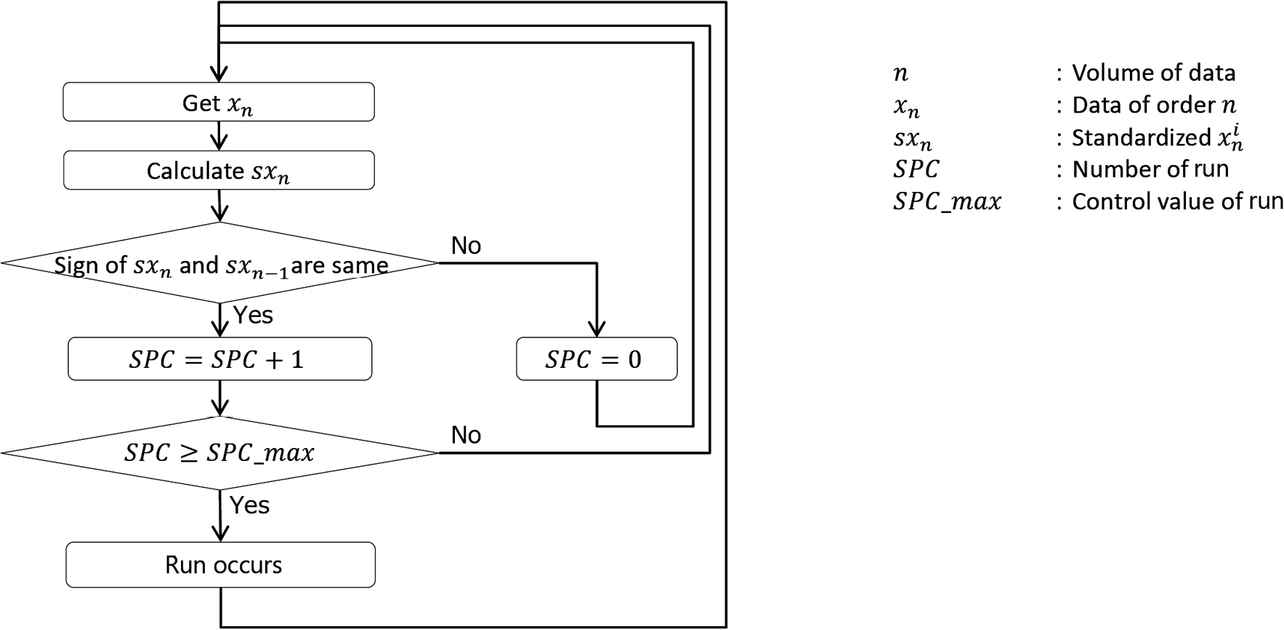
In this flow, sxn is used as a value necessary to extract occurrences of runs. However, sxn tends to have a greater absolute value because it deviates more from the average value (Ave) and can be used as an index for evaluating the degree of deviation from the average value for the sample.
The proposed method regards the occurrence of a run as the occurrence of a change. The occurrence of a run is used as the method for discarding past data and for starting learning anew. Fig. 7 shows the flow of the process that starts learning anew.
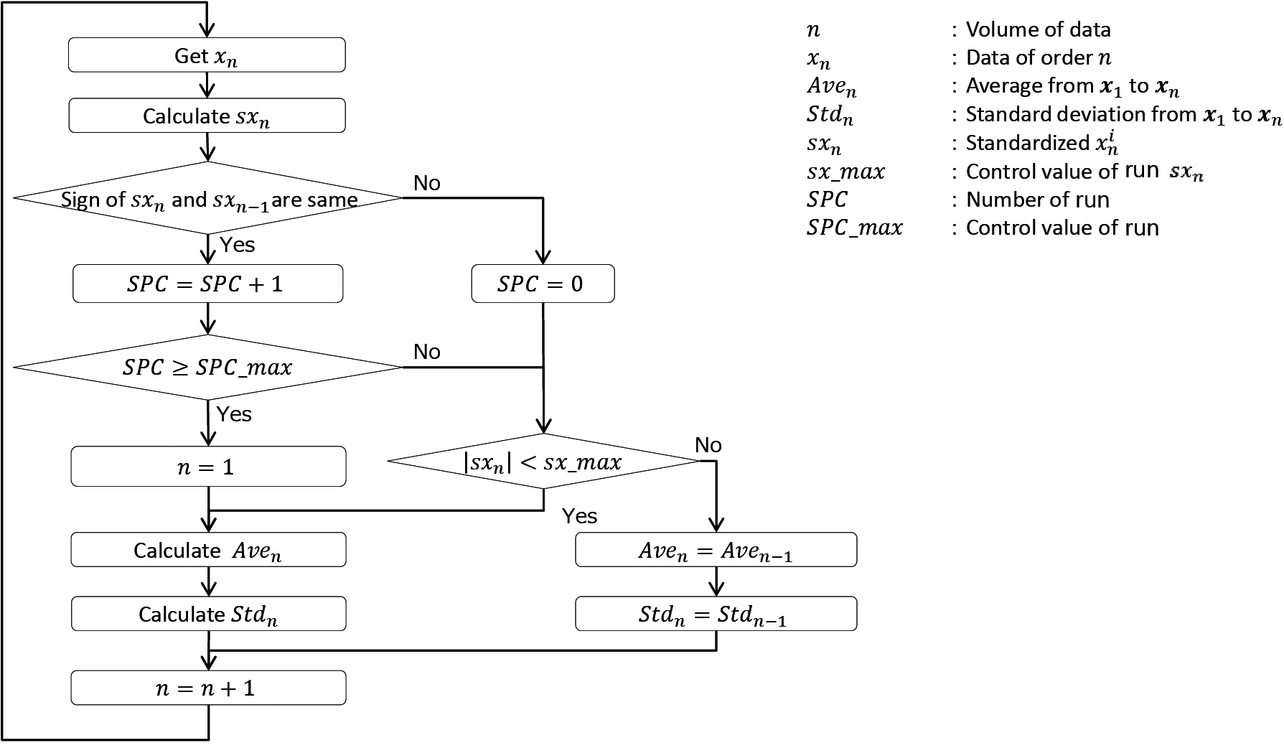
The SPC ≥ SPC _max step determines whether a run has been established. When a run has been established, n=1, thus ensuring that past learning is discarded to start sequential learning anew.
The |sxn |<sx_max step is intended to determine whether the obtained sxn is an outlier. For the criterion for determining standardized data as outliers, we set a recommended value of 3, using the three-sigma rule6) for reference. The average and standard deviation values will not be recalculated when any datum is determined as an outlier. Thus, the proposed method is designed to be resistant to the effects of outliers.
The equation for obtaining the average value by sequential learning is Eq. (3), which uses the average value Aven −1 of the data up to the n−1th datum and the nth sample value xn to obtain the average value Aven of the data up to the nth datum. Eq. (3) is derived as the sequential learning equation from the commonly known average value formula, where Ave0=0:

Before deriving the equation for obtaining the standard deviation by sequential learning, the equation for obtaining the covariance by sequential learning is derived. For the variables l and m, the covariance of the samples up to the nth one is expressed as  (
( ). When derived from the commonly known covariance formula, the sequential learning equation is given as Eq. (5). The derivation goes as follows:
First, the commonly known formula for is Eq. (4):

where

Hence,

is obtained as the sequential learning equation for obtaining the covariance.
The variance is for when m=l in the covariance equation. When the variance of the samples up to the nth one is expressed as Varn , the equation for calculating Varn by sequential learning is given as follows from Eq. (5):

where Var0=0.
A standard deviation is the square root of variance. When the standard deviation of the samples up to nth one is expressed as Stdn , the equation for calculating Stdn by sequential learning is given as follows from Eq. (6):

where Std0=0.
When the average value and standard deviation obtained by sequential learning are used, the method of sequentially standardizing data7) is given as Eq. (8), where sxn is the standardized nth sample value:

3.2 Method for cases with multiple variables
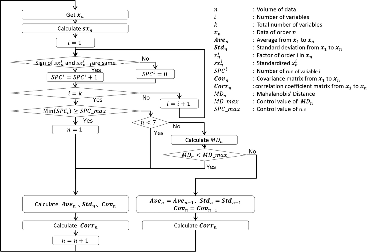
The preceding subsection presented the method for cases with a single variable. Fig. 8 shows a flowchart for a version extended to support cases with multiple variables.
3.2.1 Mahalanobis distance
In the preceding subsection, an index denoting the degree of deviation from the average value is used and with another index, sxn , used as a value for enabling a method resistant to the effects of outliers. For cases with multiple variables, the proposed method uses a Mahalanobis distance as a value with the role of sxn .
Mahalanobis distances are, for example, the lengths of arrowhead lines in Fig. 9 and represent the distances between the reference point and the respective samples. Fig. 9 uses as an example a point in a region densely populated with samples without foreign matter as the reference point. In actual calculations, the average values of the respective variables in the sample set used for learning are the reference point coordinates.
When using the Mahalanobis distance in our approach, the average value and standard deviation must first be sequentially learned for each variable, similarly to cases with a single variable. Besides, the covariance must also be sequentially learned. The equation for calculating the covariance by sequential learning is Eq. (5) above.
The equation for obtaining the correlation coefficient  from the covariance is Eq. (9):

Considering that it is convenient for manufacturing sites that a control value remains unchanged regardless of the change in the number of variables, we adopted the definitional equation5) in the MT method for quality engineering as the equation for obtaining the Mahalanobis distance. The formula for Mahalanobis distance (MD) is given as Eq. (10), where sxn is the nth sample’s data and represents the vector xn as a vector standardized for each variable. If not xn but sxn is used, the covariance matrix will be replaced with a correlation coefficient matrix8). Hence, the correlation coefficient matrix Corrn−1 created using the data for the samples up to the n−1th one is used.

For cases with two variables, the inverse matrix portion included in Eq. (10) is given as follows:

With the following formula:

Eq. (11) can be rewritten as follows:

The data in Figs. 2 and 3 are for a case with two variables. In the experiment on the proposed method in Section 4, this formula is used to calculate the inverse matrix portion.
Note that If n≤3, the Mahalanobis distance cannot be calculated for the following reasons:
- When n=1: No data available from the preceding cycle.
- When n=2: The data from the cycles up to the preceding one are one sample’s worth of data with which the correlation coefficient cannot be calculated.
- When n=3: The data from the cycles up to the preceding one are two samples’ worth of data, resulting in a correlation coefficient of 1, with which the inverse matrix cannot be calculated.
Therefore, theoretically, if n≥4, the Mahalanobis distance can be calculated. However, in our approach, an algorithm that calculates the Mahalanobis distance when n≥7 is used and expressed as “n<7” in the flowchart. This condition is specified because a small sample size may result in an underestimated standard deviation. With a small standard deviation, new samples are more likely to be determined as outliers. Our algorithm is designed not to use any data of samples determined as outliers for sequential learning. As a result, an underestimated standard deviation may be used indefinitely without end, and non-outlier samples may continue to be determined as outliers.
With this point taken into consideration, the flowchart does not contain “n<4” but “n<7,” which is a temporary value. If this value is too small, non-outlier samples will likely be erroneously determined as outliers. On the other hand, if the value is too large, a risk occurs of increased samples that do not get their Mahalanobis distance calculated.
3.2.2 Run for cases with multiple variables
For cases with a single variable, as in the preceding subsection, a run is defined by the rule that standardized values occur consecutively on either the positive or negative side. The proposed method defines a run for cases with multiple variables as follows: first, the respective variables are checked individually to determine whether a run has been established; then, if a run has been established for either variable, the run is defined as a run for the multiple variables. This part corresponds to a step given as follows in the flowchart:

3.2.3 Outlier determination method
For outlier determination, we adopted the Mahalanobis distance as the index for multivariate outlier determination. For the criterion value, we set a recommended value of 4 based on the determination criteria in the MT method9). Excluding data of samples identified as outliers from sequential learning, we made our outlier determination method resistant to the effects of outliers.
4. Experiment
This section discusses the results of applying the proposed method to the data from the packaging machine presented in Section 2.
4.1 Run control value adjustment
Fig. 10 is a graph showing the calculation results for the average value Aven as red dots superimposed on the data xn from Fig. 2. The average value Aven showed a significant change after Cycle 212, which is a calculation result as intended. However, as with the parts encircled with yellow dotted lines in Fig. 10, some parts other than those after Cycle 212 also showed the average value changing discontinuously. The changes during cycles other than Cycle 212 were relatively short-lasting.
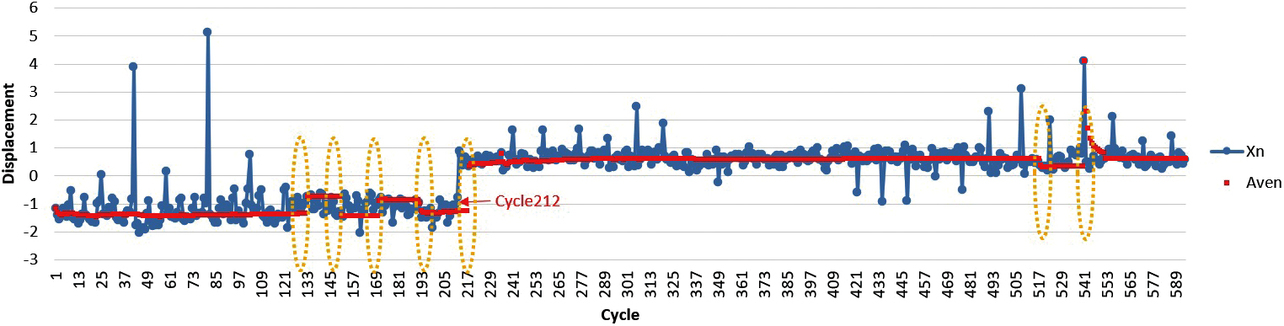
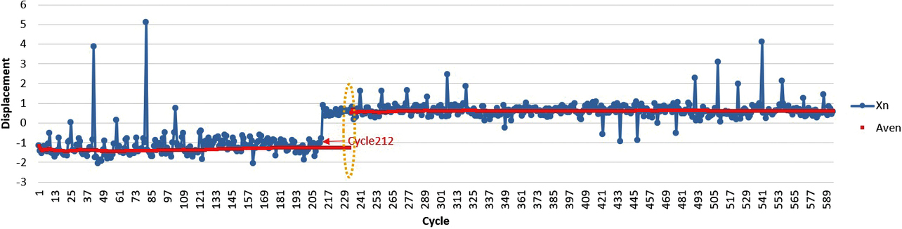
Here, the proposed method can serve two purposes: detecting changes, including relatively short-lasting ones, or ignoring relatively short-lasting changes. It is the latter that is required by the challenges presented in Section 2. Therefore, what follows is based on the method that ignores relatively short-lasting changes. Hence, the run length should probably be set to greater than 9. Fig. 11 shows a case with the run control value changed to 25 on a trial basis. With this change, the average value showed significant discontinuous changes only after Cycle 212.
This paper has revealed the importance of run control value adjustment. When this control value is set small, the average value changes discontinuously more frequently, resulting in increased indeterminable samples (=6×number of change points) because determination is impossible during the “n<7” period immediately after a change. On the other hand, setting this control value large results in a large sample size necessary to determine whether a run has been established (=run control value×change point). For this sample set, the pre-change criteria apply, making proper determination impossible. This relationship can be estimated as shown in Table 1, where the total value of indeterminable samples and samples to which the pre-change criteria apply is the smallest when the run control value is 25. This observation shows that the run control value needs to be adjusted to be not too large or too small.
| Run control value |
Number of change points |
Indeterminable samples |
Samples to which pre-change criteria apply |
Total |
|---|---|---|---|---|
| 9 | 7 | 42 | 63 | 105 |
| 25 | 1 | 6 | 25 | 31 |
| 50 | 1 | 6 | 50 | 56 |
| 75 | 1 | 6 | 75 | 81 |
4.2 Results comparison with the conventional methods
The proposed method was implemented and compared with conventional methods. The conventional methods used for comparison were based on the following two types of learning: batch learning and sequential learning. The point common in both is that the Mahalanobis distance MD is calculated.
The proposed method was implemented with the run-length criterion value set to 25 based on the results from Subsection 4.1. The batch learning-based method uses the samples from Cycle 1 to Cycle 24 as the learning data and performs MD calculation based on the average value, standard deviation, and correlation coefficient for these data. The sequential learning-based method calculates and updates the average value, standard deviation, and correlation coefficient sequentially from Cycle 1 and uses these values to perform MD calculation. Unlike the proposed method, this method does not default to n=1 at the occurrence of a run.
Fig. 12 shows the results. “Without foreign matter” refers to a group of samples with no foreign matter jammed in. “With foreign matter” refers to a group of samples with foreign matter jammed in. The three methods were compared regarding the MD distributions for these groups. The batch and sequential learning-based methods showed a significant overlap between the distributions with and without foreign matter. In contrast, the proposed method showed relatively separate distributions.
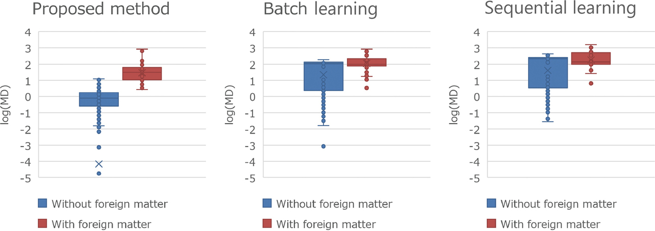
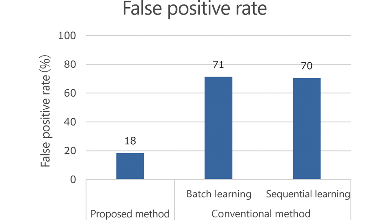
For each method, Fig. 13 shows the false positive rate, in other words, the proportion of samples exceeding the minimum Mahalanobis distance MD set as the criterion for samples with foreign matter from among those not containing any. That is to say, the figure shows the error rates for cases with a criterion specified to ensure that samples with foreign matter were determined defective. The proposed method showed a rate of 18%, an approximately 50 percent improvement from the rates of around 70% shown by the two conventional methods. Thus, the proposed method has been proven effective for the data fluctuations shown in Figs. 2 and 3.
5. Conclusions
Data from manufacturing sites may exhibit abrupt changes. How to accommodate such changes poses one of the challenges in applying machine learning to manufacturing sites.
We applied sequential learning algorithms and the idea of the stable state index in control charts to the above challenge to propose an anomaly determination algorithm that can automatically track and adapt to changes. Applying this algorithm to the data from an experiment using a packaging machine, we confirmed that the proposed method showed a false positive rate of 18%, an approximately 50 percent improvement from the rates of around 70% shown by the two conventional methods used for comparison.
In implementing our approach, the task of run length setting is left to the user. Our approach performs automatic run-based fluctuation detection and automatically obtains learning data by sequential learning. However, this adjustment also faces the challenge of making settings automatically to suit the nature of the phenomenon of interest.
Our approach assumes situations where average values are maintained for a certain period before and after abrupt changes that may occasionally occur. As such, our approach cannot handle phenomena that continue changing constantly without average values maintained for a certain period. For these phenomena, the challenge is to devise an alternative algorithm. Building also on the remaining challenges above, we will consider incorporating the technology presented herein into OMRON’s controllers and other ways of contributing to solving customers’ challenges.
References
- 1)
- OMRON Corporation. “Solution AI,” (in Japanese), https://www.fa.omron.co.jp/solution/technology-trends/ai/ (Accessed: Dec. 1, 2022).
- 2)
- R. Mizoguchi and T. Ishida, Artificial Intelligence, (in Japanese), Ohmsha, Ltd., 2013.
- 3)
- Y. Unno, D. Okanohara, S. Tokui, and H. Tokunaga, Online Machine Learning, (in Japanese), Kodansha Ltd., 2015.
- 4)
- Y. Sakamoto, Y. Nakamura, and M. Sugioka, “A Case Study of Real-time Screw Tightening Anomaly Detection by Machine Learning Using Real-time Processable Features,” (in Japanese), OMRON TECHNICS, vol. 55, no. 1, pp. 35-44, 2023.
- 5)
- M. Miyagawa and Y. Nagata, Exploration into the Taguchi Method, (in Japanese), JUSE Press, Ltd., 2022.
- 6)
- Japanese Standards Association, JIS Handbook Quality Control, (in Japanese), Japanese Standards Association, 2022.
- 7)
- D. Ogihara, Approach to Data Analysis and Guide to Introducing AI/Machine Learning, (in Japanese), Johokiko Co., Ltd., 2020.
- 8)
- Y. Wakui and S. Wakui, Illustrated Guide to Multivariate Analysis, (in Japanese), Nippon Jitsugyo Publishing Co., Ltd., 2001.
- 9)
- K. Tatebayashi, Introduction to MT Systems, (in Japanese), JUSE Press, Ltd., 2008.
The names of products in the text may be trademarks of each company.