


Development of a Method for Estimating the Range of Electrical Disturbances Using Product-scale Simulation and Dynamic Search
- System Simulation
- Causal Model
- CAE Application Technology
- Adaptive Design of Experiments
- Range Estimation Method
Products are required to have robust quality to operate stably against disturbances in various usage environments. To satisfy such requirements, it is necessary to verify operation under a variety of different conditions and to eliminate conditions that cause unstable operation, which is where CAE technology is effective. However, it is difficult to analyze electrical behavior at the product level using conventional circuit simulation, and the evaluation of electrical disturbances has been conducted mainly on actual equipment.
In this study, we developed a method to efficiently estimate the conditions of disturbances that make product behavior unstable from a wide range of conditions by using system simulation technology that can analyze product-scale electrical behavior and a dynamic search method and confirmed its effectiveness through verification of actual equipment. By utilizing this technology, it is expected to be effective in preventing the false negatives of disturbance conditions that cause unstable behavior, which was conventionally judged on an individual basis.
1. Introduction
Market environments have diversified in recent years. So have the surroundings to which products are exposed. In this context, products should have robust quality to operate stably against disturbances due to a variety of different environmental fluctuations. Electrical products are prone to unstable operation due to electrical disturbances, such as sudden voltage/current fluctuations, and should be designed to be immune to them.
Measures implemented against disturbances during development include logical verification and empirical design. Moreover, developments rely on experimental verification for evaluations to check quality. In evaluations, past evaluation results and the expertise of experienced designers provide the basis for guessing disturbance conditions that make the product unstable. Under these conditions, physical prototypes are subjected to electrical disturbances and inspected for behavior. The current practices are stuck in this reality.
With these circumstances unchanged, the following problems will occur:
- Worst-case conditions the designer assumes cannot be verified on the desktop to be correct, resulting in false negatives for unstable behavior.
- The product differs from past models in disturbance conditions or ranges for instability, resulting in false negatives for unstable behavior.
- With unstable behavior addressed mainly by the experimental cut-and-try approach, issues other than addressed conditions may deteriorate unnoticed, resulting in false negatives for unstable behavior.
In this situation, the challenge is to accurately identify and address behavior unforeseeable at the design time or unstable conditions against disturbances within a limited verification period. A non-experimental verification method capable of inspecting a wide range of circuit behavior on the product-level scale is necessary to solve the above-mentioned challenge.
This paper reports on a utilization technology that combines system simulation technology and a dynamic condition search method to detect the range of disturbance conditions for unstable behavior accurately. Section 2 explains the challenges in circuit simulation and condition range estimation and presents a method for overcoming these challenges. Section 3 describes the system simulation for reproducing the product-scale electrical behavior constructed. Section 4 describes the analysis method of estimating, based on simulation results, the range of disturbances that may affect product operation. Then, Section 5 presents the findings obtained. Finally, Section 6 wraps up a summary and discusses the future prospects.
2. Proposal for an efficient method to search for disturbance conditions on a product scale
2.1 Current situations
This subsection discusses circuit simulation technology as the conventional desktop verification method of inspecting electrical behavior and the current state of condition searching in the effective use of system simulation.
2.1.1 Current state of circuit simulation technology
Circuit simulation is a technology for reproducing electrical behavior on the desktop. This paper uses the term “circuit simulation” as a generic name for tools and analysis methods for efficiently designing and analyzing electric circuits. A typical example of circuit simulation is the Simulation Program with Integrated Circuit Emphasis (SPICE).
In circuit simulation, an electric circuit model is constructed based on a circuit diagram to reproduce the entire circuit, including the characteristics of and the wiring between the on-board electrical parts. Then, an analysis engine that suits the purpose of the verification is used to obtain simulated electrical waveforms from the model. A common practice in verifying behavior against electrical disturbances is to obtain the waveform of each section in the circuit over the lapse of time using transient analysis.
2.1.2 Current state of condition range estimation technology
It is a common practice in system simulation utilization to search parameter ranges at once. Mainstream methods are static search methods, including an exhaustive search (grid search) and a parameter search using statistical thinning of conditions (design of experiments (DoE)). Given that the analysis time per search×the number of searches equals the total time for range searches, one of the critical points in using this technology is to specify the number of searches, considering the trade-off between the total time and the available resolution range.
2.2 Challenges
In relation to the current situation explained in Subsection 2.1, this subsection describes the challenges in searching the range of disturbance conditions on a product scale.
2.2.1 Challenge of simulating circuits on a product scale
With the current circuit simulation technology, it is impractical to analyze the behavior of an entire product against disturbances. Let us assume that the entire circuit of a product is the target of analysis. It would then be necessary to handle numerous models of electrical parts or devices. The electric circuit model would become larger in scale with an increasing number of parts, resulting in an increased analysis time. Moreover, the analysis would converge poorly in some cases involving numerous wired electrical parts, leaving the circuit behavior unanalyzed. Especially in the case of models containing a feedback circuit (closed loop), such as a control circuit, a particularly poor convergence would result because of the numerous complicated devices with nonlinear electric characteristics. Thus, it is impractical to analyze the entire circuit of the product. The utilization of circuit simulation remains mainly limited to the partial verification of characteristics with the target of analysis limited to a specific circuit block.
2.2.2 Challenge of condition range estimation
Even if the challenge in the previous sub-subsection were overcome by enabling circuit simulation on the product-level scale, it would remain challenging to search the range of disturbances that would cause unstable behavior. To search for a target condition for a product-level, large-sized model, one must analyze the product’s behavior using exhaustive combinations of product operation and disturbance conditions. As a result, the required analysis time will increase exponentially with an increasing number of parameters as analysis conditions, making it impossible to use this estimation with the limited verification period upstream of design.
Therefore, when the aim is to identify the range of disturbances that affect product operation based on the behavior analysis results on the product-level scale, the challenge is to develop a utilization method for efficiently detecting unstable conditions from a wide search range.
2.3 Principles for solving the challenges
To solve the challenge presented in 2.2.1, we incorporated a causal model into the conventional circuit simulation to avoid an increased computational scale so that we could develop a system simulation technology that enables operation analysis on the product-level scale.
Besides, to solve the challenge presented in 2.2.2, we introduced a method for intensively searching the range of conditions for unstable behavior while dynamically changing the search condition. At the same time, we linked the system simulation technology with a dynamic condition search method to allow estimating the range of disturbances where the product operates unstably.
2.3.1 Addition of a causal model
We planned to add a causal model to enable analysis of the behavior of an entire product. The electric circuit model in the conventional circuit simulation is a method that describes everything using physical model elements known as noncausal models. In the electric circuit shown in Table 1, the resistors, capacitor, power supply, and the like fall under the definition of model elements. The noncausal model obeys the laws of physical equilibrium (e.g., Kirchhoff’s law) and hence features excellent compatibility with electric circuits.
| Aspect | Noncausal model |
|---|---|
| Concept | The relationship between elements is represented as an equation that analyzes the whole model. |
| Examples of connection methods | 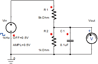 |
| Model elements | Resistors, coil, capacitor, power supply, etc. |
| Feature | Capable of directly representing physical equations and hence highly compatible with electric circuit models. |
| Advantage | Able to model physical structures to analyze electrical behavior with high accuracy to meet the laws of physical equilibrium. |
However, when the circuit of interest is a control circuit, such as a feedback circuit, an attempt to construct the functions of its constituent devices in the noncausal model elements will lead to a massive number of elements. Hence, a causal model suits the purpose and converges well without requiring much time for iterative calculations: it can concisely represent the input-output signal relationship specified by the devices in the control circuit shown in Table 2 and the order of operations1).
| Aspect | Causal model |
|---|---|
| Concept | Performs analysis using successive substitution between the elements in an input-output relationship. |
| Examples of connection methods | 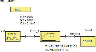 |
| Model element | Gain, adder, transfer function, etc. |
| Feature | Capable of explicitly showing calculation sequences and hence highly compatible with control models or programs. |
| Advantage | Able to achieve better convergence than the noncausal model and needs less time for iterative calculations. |
Note that a causal model determines the required level of detail for each model element and performs conversion of the function of the complicated equivalent circuit represented in circuit simulation using mathematical expressions, data tables, and state transitions. More than one causal model that uses their combination to express a complicated function with a small number of elements is used to obtain a model that balances the product-level model size and the accuracy sufficient to represent electrical behavior.
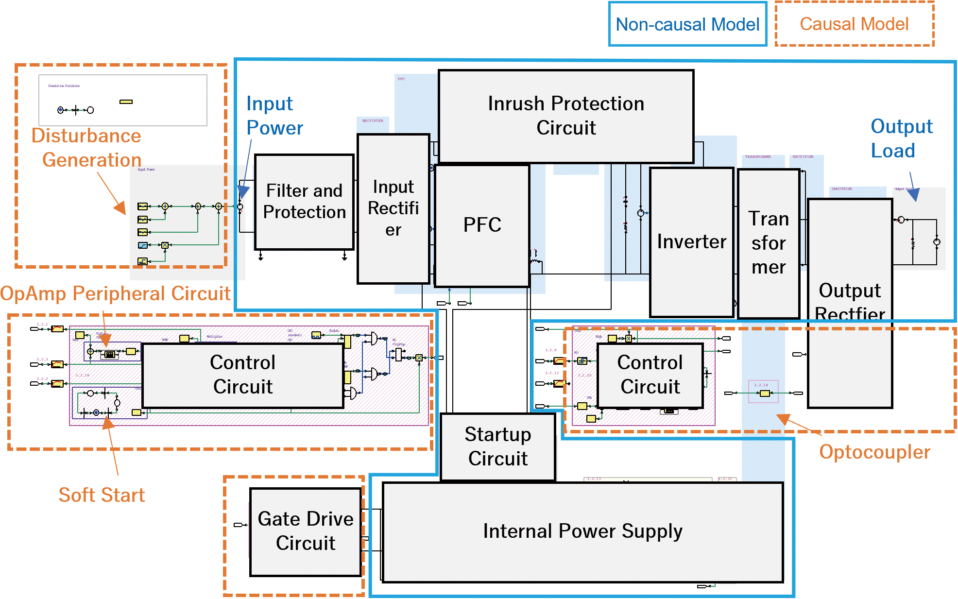
Therefore, the optimal configuration is to use the conventional circuit model (noncausal) for the circuit sections necessary to achieve the product’s primary function and the causal model for the section constituting the product’s control circuit. Hence, we implemented this configuration. In this paper, a model that combines a circuit model and a causal model is called a system model. This model enables analyzing the electrical behavior of an entire product. Refer to Section 3 for the specific results of model construction.
2.3.2 Dynamic search for instability conditions
We planned to implement a dynamic search method that efficiently searches for instability conditions from a wide search range. Dynamic search is a method that uses the information from a condition search to determine subsequent conditions one by one and to proceed with the search.
For comparison, let us discuss the static search method described in sub-subsection 2.1.2. In static search, conditions are collectively specified before analysis to analyze each. With the conditions to search for being planned beforehand, it is easy to implement the static search method. Fig. 1 shows an example of searching a fault range based on two conditions. The left-side figure shows the simplest search method (exhaustive search) that exhaustively searches for each condition at regular intervals. Meanwhile, the right-side figure visualizes search points subjected to DoE (statistical thinning of conditions), which uses a limited number of conditions to search a wide range.
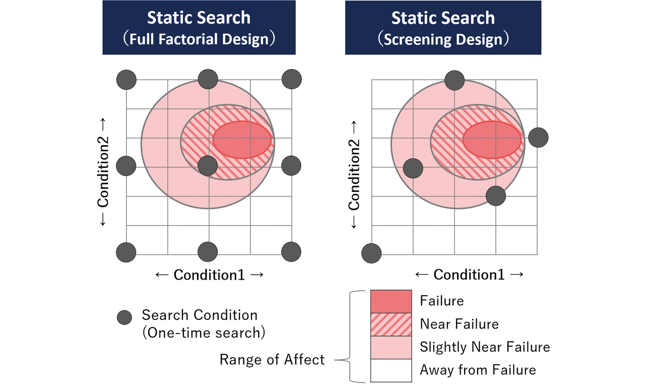
In both cases, however, false negatives occur for a fault if the fault condition exists between the pre-planned search points, as shown by the fault range in the figure.
As regards this problem, let us explain with reference to Fig. 2, the dynamic search method of proceeding with search while determining conditions one by one. The first step is to search for a search point (Point 1) extracted from a wide range. In this range, a point closer to the fault range is located. Next, another search point (Point 2) is set around the located point to run a similar search in a narrower range. In the narrower range, yet another search point (Point 3) is set around a point even closer to the fault range to run an additional search. In this way, the method performs searching while dynamically changing the search condition to identify conditions for instability accurately and efficiently.

For the results of analyzing a specific range of disturbance conditions by dynamic search, refer to Section 4.
3. System simulation technology to reproduce electrical behavior on a product scale
3.1 Model configuration obtained
This subsection describes the system model configuration that enables operation analysis on the product-level scale. Circuits for handling the power in a product or circuit sections related to the power supply system are represented with noncausal models as electric circuits. On the other hand, the section constituting the product’s control circuit and those outside the product responsible for electrical disturbances are represented with causal models. A model integrating both models is used for an overall transient analysis. Fig. 3 below shows a typical model configuration for an example of a switching power supply:
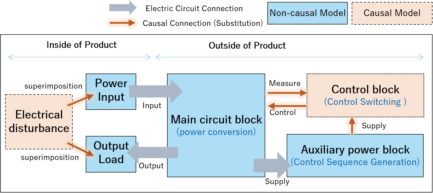
We defined the selective use of causal and noncausal models for our proposed technology. As a basic rule, we used noncausal models to make representations. We used causal models only when any of the following three criteria was the case:
- A circuit that uses current or voltage as a signal without regard to the current-voltage relationship. Examples include voltage transmission-type analog circuits or digital circuits for logical operations of MPUs and memory.
- A circuit that uses a mathematical expression or data table to express input-output relationships where the output varies according to the input. Examples include op-amp application circuits whose input-output transfer function can be formulated or photo-couplers with a well-defined data table for the input-output relationship.
- A case of reducing temporal variation patterns of characteristics. Examples include sequences of electrical disturbances, such as voltage dips/power interruptions specified in JIS C 61000-4-112).
Using an analysis tool able to represent causal and noncausal models on the same model, we performed a transient analysis on a model constructed according to the above configuration and criteria, thereby successfully analyzing the behavior of an entire product. From here on, this analysis is called system simulation. For the example of analysis discussed below, we used ANSYS Twin Builder 2023 R1 as the analysis tool.
3.2 Specific model for product-scale behavior analysis
Fig. 4 shows a system model of a switching power supply, which we constructed using our proposed technology. Each circuit constituting the basic configuration of the switching power supply3) was described into a causal or noncausal model according to the selective use defined in Subsection 3.1. Using causal models, we successfully reduced the model size.
An electric circuit model representation of, say, an operational amplifier and its peripheral circuit would require several tens of model elements, as shown in Fig. 54). The use of causal model representations allowed us to configure our model with the three elements of an adder, a data table representing the nonlinear gain, and a transfer function expressing the frequency characteristics.

3.3 Results of reproducing the steady-state behavior of the product
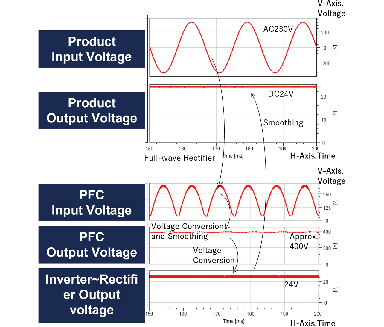
This subsection presents the analysis results for the drive waveform of a switching power supply as an example of product-scale behavior analysis enabled by our proposed technology. As shown in the top pane of Fig. 6, we observed that the switching power supply circuit converted an AC voltage input into a DC voltage output. This conversion is the circuit’s primary function of AC-DC power conversion itself. Moreover, as shown in the bottom pane of Fig. 6, the PFC input section showed a full-wave rectified waveform with the product input voltage rectified. The PFC output section showed a constant voltage waveform converted from this waveform. The inverter-to-rectifier section output showed the waveform of the voltage stepped down in the PFC output section.
Let us next explain that our model produced a proper steady-state waveform. The PFC circuit, whose control state varied depending on the input and output conditions to show different waveforms, was specified as the circuit section usable for proper inspection of the steady-state waveform. PFC circuits perform switching operations using rectangular waves to keep a constant internal voltage. It is known that these circuits cause switching voltage waveforms to vary depending on the input voltage and the output load. Affected by most of the circuits in the product, this behavior is hard to model. In our verification, we examined the switching voltage waveform of the PFC circuit under the minimum and maximum input voltage and output load as the steady-state added with no disturbances.
Figs. 7 and 8 show the analysis results for the waveforms of the steady-state switching voltage. Fig. 7 shows waveforms under two different conditions, one being 0% load (no load) and the other 100% load (rated load), with the input set to minimum. Fig. 8 shows the results under the two conditions of the input voltage set to the specified minimum and maximum values under the rated load. These analysis results reproduce the switching-induced rectangular waves, confirming that the output waveforms occurred correspondingly to the input voltage and the output load capacity.
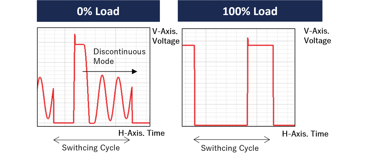
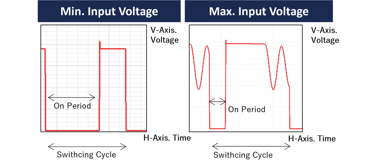
The switching power supply used in the verification is equipped with a step-up chopper-type PFC circuit. From Fig. 7, the circuit was in discontinuous-mode operation with an oscillating waveform when under 0% load and in continuous-mode operation with a continuous rectangular waveform when under 100% load. From Fig. 8, the ON period was long under the minimum input voltage and short under the maximum input voltage. These results agree with the features of step-up choppers in general5) and seem reasonable.
These analysis results confirm that our model reproduced the primary function of the switching power supply and correctly analyzed the behavior of the entire product.
3.4 Results of reproducing the behavior of the product under disturbances
This subsection explains the results of reproducing the product’s behavior against disturbances. We applied a disturbance waveform to the input section of the switching power supply to confirm that our model reproduced waveforms of the product’s internal transient behavior similar to those obtained by measurement. Sub-subsection 3.4.1 below shows the disturbances applied. Sub-subsection 3.4.2 compares the measured and analyzed results.
3.4.1 Disturbance waveform applied to the product
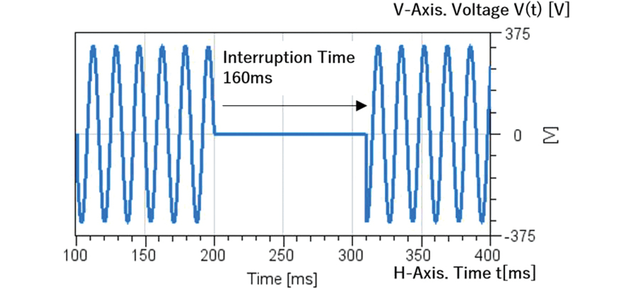
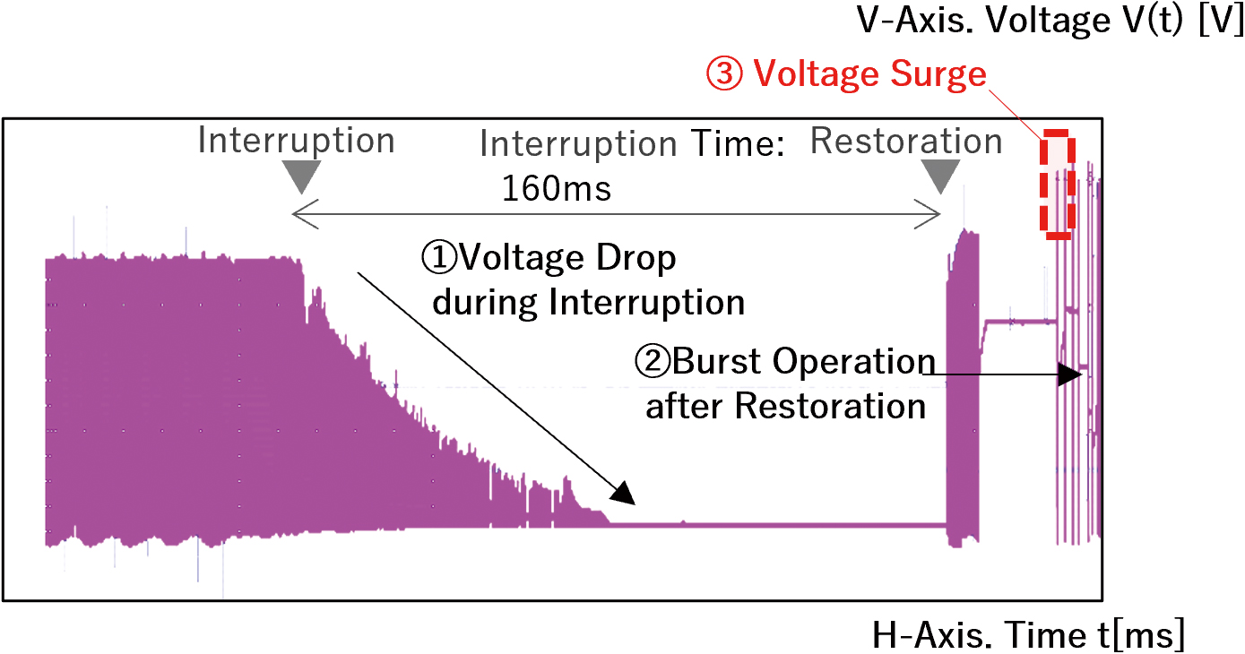
One of the typical disturbances to products with a power supply input section is power interruptions of input power supplies. JIS C 61000-4-11 specifies the following voltage fluctuation test procedure: after keeping the input voltage at a normal level, keep it low for a certain period and then raise it back. The phrase “power interruption” refers to a voltage drop of 100% in particular. As shown below in Fig. 9, our analysis applied a power interruption of 160 ms as a disturbance to a switching power supply with an operating voltage of 230 VAC.
3.4.2 Measured waveform of transient behavior vs. analyzed results
As a result of applying the disturbance shown in the previous sub-subsection, similar behaviors appeared in the measured and analyzed results. To verify the switching power supply, we used two versions of samples: a standard sample with no transient voltage stress from disturbances and an unprotected sample with the countermeasure component intentionally removed. This sub-subsection discusses the results of applying a disturbance to each sample.
As shown in the second row of Table 3, the standard sample showed a decrease in internal switching voltage due to a power interruption and then a rise back to the original voltage level upon the end of the power interruption. The results for the standard sample showed that it operated stably against the power interruption-induced disturbance.
| Product | Full/enlarged | Analyzed results | Measured results |
|---|---|---|---|
| Standard sample | Switching voltage (full) | 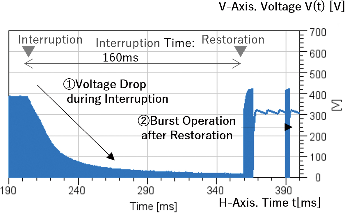 |
 |
| Unprotected sample | Switching voltage (full) | 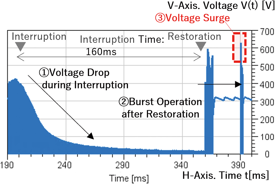 |
 |
| Switching voltage (enlarged) | 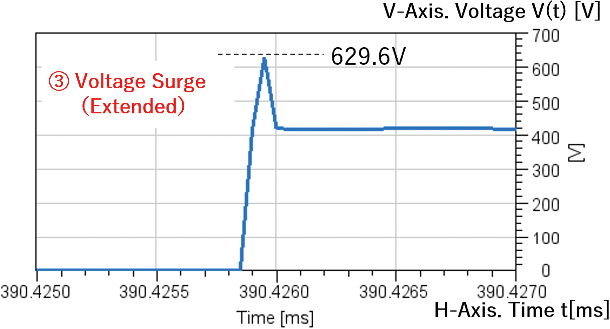 |
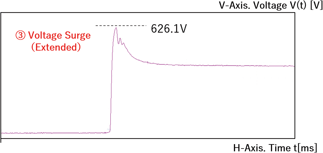 |
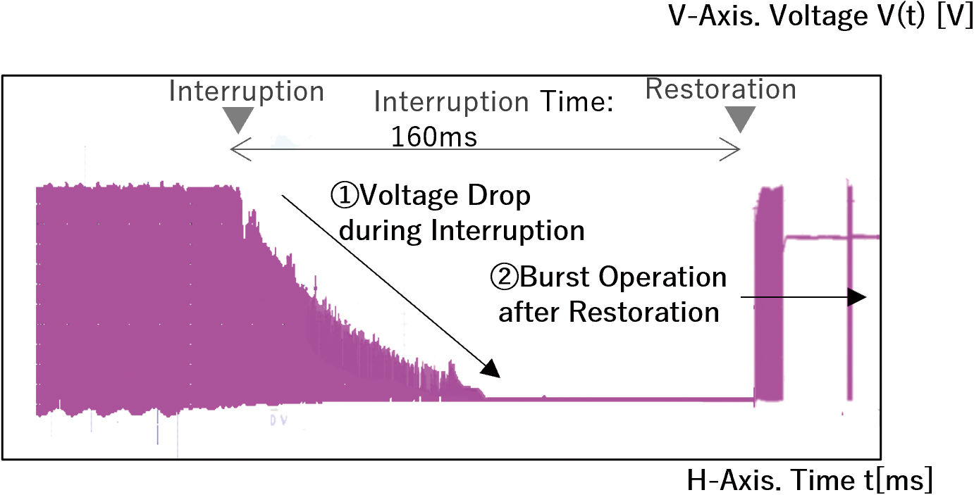
On the other hand, as shown in the third and fourth rows of Table 3, the unprotected sample showed a behavior involving an excessive rise in switching voltage at the recovery from the power interruption in both experimentally measured and analyzed results. The critical features of this behavior were the following three phenomena (1) to (3):
- (1) The switching voltage drops during the power interruption period.
- (2) At the recovery from the power interruption, the dropped switching voltage returns to the original level in (1), followed by cycles of intermittent operation.
- (3) A surge occurs in the switching-voltage waveform during the intermittent operation at the recovery from the power interruption.
The waveforms for these three phenomena show the same features (1) to (3) in the measured and analyzed results. Moreover, the maximum voltage surge value was similar between the measured and analyzed results. Therefore, these results confirm that the transient behavior of the product against disturbances was reproduced.
4. Method of dynamically searching the range of disturbances for unstable behavior based on simulation results
4.1 Overview of the method for extracting an input range from a model
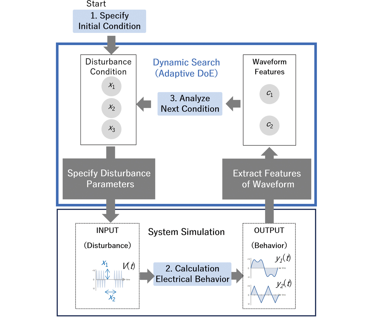
This method consists of two parts: quantifying the inputs and outputs to and from the model-based analysis discussed in Section 3 and applying adaptive design of experiments (DoE), which repeats dynamic searches to determine subsequent inputs based on outputs.
Let us first explain the part of quantifying the inputs and outputs to and from the system model. To use the system model in adaptive DoE, one must define the inputs to the model as parameters to quantify the model’s output waveform. The inputs to the system model were the parameters expressing the features of a disturbance waveform. In the case of a power interruption-induced disturbance, the power interruption time [ms] shown in sub-subsection 3.4.1 or the voltage drop rate [%] during the power interruption period corresponds to the input parameters to the system model.
The outputs from the system model were the waveform feature quantities obtained from the model analysis results. The electrical waveform feature quantities were extracted by mathematical operations. For example, the maximum, minimum, and mean values correspond to functions that extract feature quantities.
Let us next move on to the adaptive DoE that enables dynamic condition search. We adopted Lipschitz sampling6), the adaptive DoE algorithm implemented in modeFRONTIER 2022R3, ESTECO’s optimization software, as the dynamic search method for our proposed method. A range search must not only find unstable conditions but also identify a range, including the boundary between the occurrence and non-occurrence conditions for unstable behavior. Therefore, Lipschitz sampling, which intensively searches for conditions for highly variable quantified outputs, was used as the dynamic search algorithm. Lipschitz sampling is a valid method of narrowing down the occurrence areas of changes that are important for the behavior of the modeled phenomenon.
Fig. 10 shows a series of steps for enabling the above-mentioned dynamic condition search. The first step was to specify the initial disturbance condition (Step 1). The next was to obtain the waveform for behavior analysis results by system simulation (Step 2). What followed was to evaluate the obtained waveform feature quantities by adaptive DoE and specify the next analysis condition (Step 3). Then, Steps 2 and 3 were repeated in a series of cycles to search efficiently for the range of disturbance conditions.
4.2 Results of searching an instability range using adaptive DoE
Regarding the system model of switching power supply presented in Section 3, this subsection explains its ability to extract the range of disturbances for unstable behavior occurrences, using as an example the behavior of transient voltage surges in the unprotected sample.
Table 4 shows the quantified indices used for searching. The parameters expressing the power interruption-induced disturbance and the product use conditions were specified as the inputs. The maximum value of the PFC circuit switching voltage was the quantified output. The search condition was the switching voltage range above 600 V, in other words, the high-stress range for the device.
| Type | Quantified index |
|---|---|
| Input | 1) Parameters for power interruption condition … Power interruption time [ms] and power interruption rate [%] 2) Parameters for product use conditions … Input voltage [V] and output load [W] |
| Output | 3) Maximum voltage for the switching section* … MAX() function * High-stress range > 600 V |
Based on the above indices, search conditions were dynamically determined to perform analysis by system simulation and obtain output data corresponding to the required number of inputs. Fig. 11 shows the results of visualizing the input-output relationship as a scatter plot. The search identified the following conditions for the voltage to reach the high-stress range for the device:
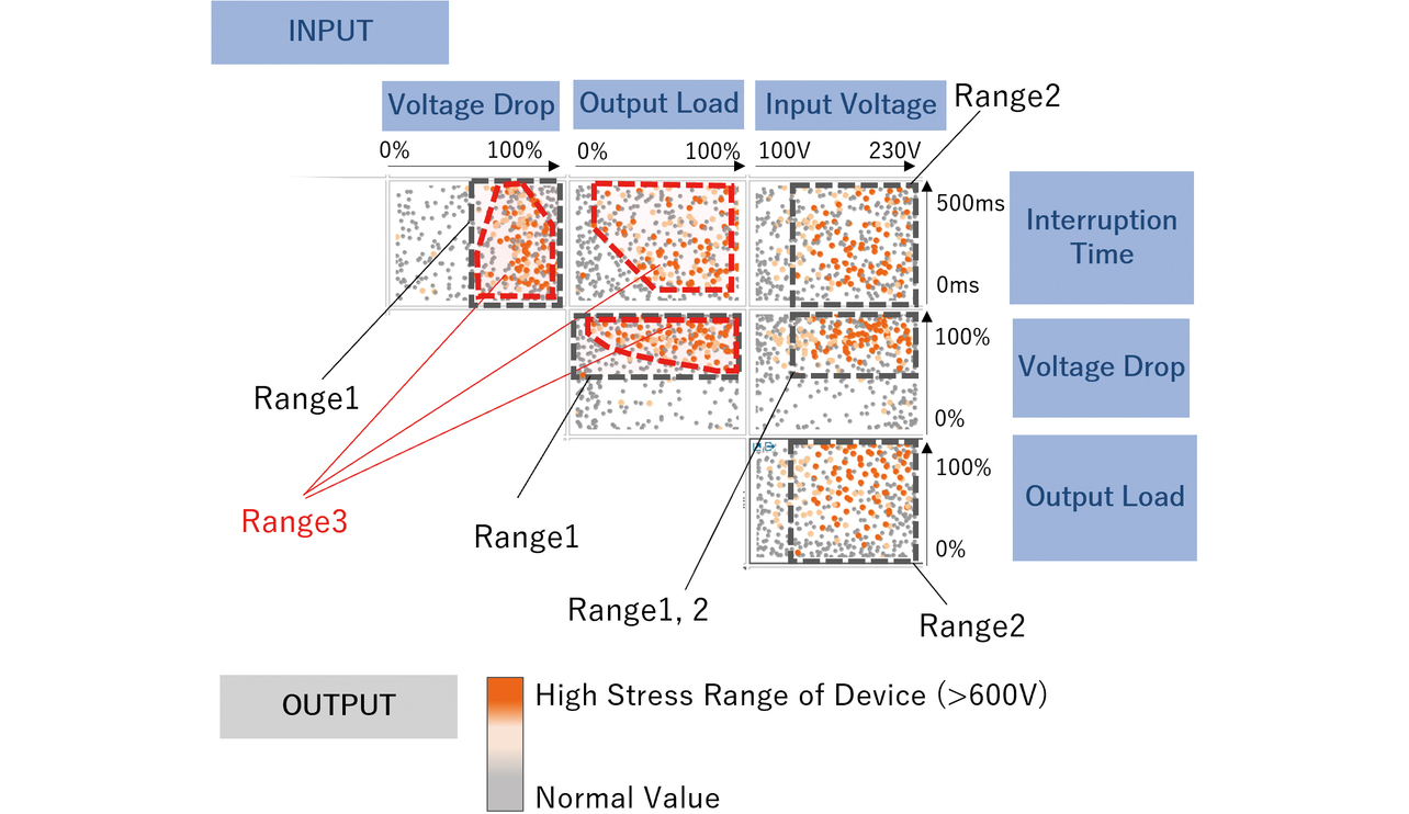
- Range 1: The high-stress range is reached when the power interruption rate is 47% or over.
- Range 2: The high-stress range is reached when the input voltage is 130 V or over.
- Range 3: In a certain range, the high-stress range is reached due to the interactions among the power interruption rate, the power interruption time, and the output load.
The analysis dataset size was N = 456, equivalent to a search with 4.6 levels per parameter in a four-parameter static search (exhaustive search). Considering that eight levels per parameter, in other words, an analysis dataset with N = 4096, would be necessary to derive a range for obtaining similar analysis results using static search, we can say that dynamic search enabled an efficient search of the range for the occurrence of unstable behavior.
At the same time, Fig. 11 shows that the high-stress ranges for the device and their surrounding areas were finely searched, while the areas under conditions for normal values were coarsely searched. These results reflect the features of the Lipschitz sampling search and visualize an accurate search for the range of conditions defined as “unstable.”
5. Effectiveness of our proposed method
5.1 Agreement between the estimated and experimentally measured ranges
This section compares the instability range estimated using our proposed method with the actual one confirmed by measurement to demonstrate the validity of our proposed method as a means of range estimation.
From the perspective of examining the need for rework at the design phase, this subsection distinguishes and calls numerically unstable and normal ranges, respectively, as follows:
- Pass … Condition in which the high-stress range for the device is or below (600 V); and
- Fail … Condition in which the high-stress range for the device exceeds (600 V).
Among the conditions searched in subsection 4.2, the simulated “Fail” ranges of the output load and the power interruption time, including interactions between them, showed a similar tendency to those obtained by measurement.
Fig. 12 shows the simulated and measured results for the maximum voltage value of the switching section. The left side shows the analyzed results, the right side shows the measured results, and each group of highlighted boxes forms a “Fail” range. The fixed conditions were a power interruption rate of 100% and an input voltage of 230 V, while the variable conditions were the output load and the power interruption time.
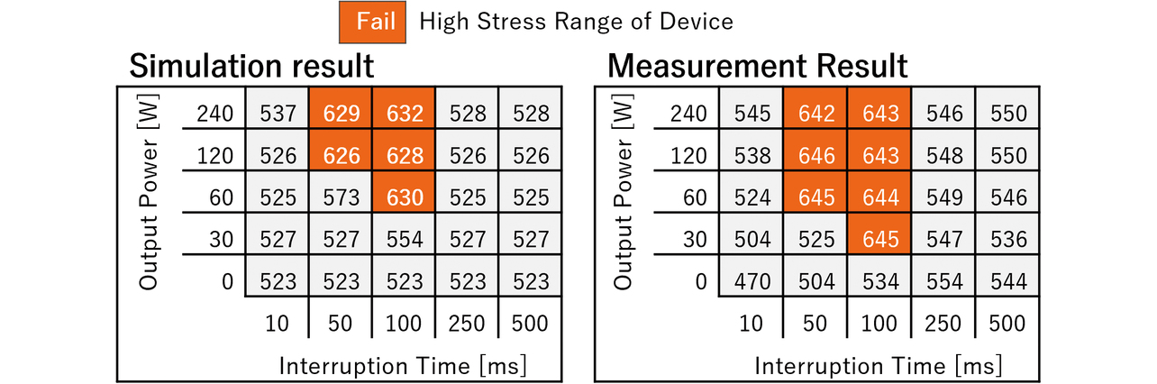
Of the 25 conditions examined, the simulation made correct pass/fail judgments for 23 conditions. Besides, the measured and analyzed results both tend to show a concentration of fails in a certain range for the power interruption time and the output load power.
The simulation made pass judgments for the remaining two conditions, while the measurement made fail judgments. The cause is that the analyzed values tend to be lower than the measured values because of the reproducibility of the electric circuit model (noncausal model). On the other hand, the simulation fully agreed with the measurement for the conditions for which it made fail judgments.
For these two perspectives, we made a comprehensive evaluation to calculate the recall and precision, two evaluation metrics of statistical analysis. As shown in Table 5, the results were that the recall was 71%, while the precision was 100%.
| Aspect | Recall | Precision |
|---|---|---|
| Concept | What percent of actual fails are correctly identified? | What percent of fails identified by simulation are actually fails? |
| Implication | Metric denoting the infrequency of false negatives for instability conditions | Metric of instability condition detection without false judgments |
| Calculation formula |
(# of conditions for fail judgment by simulation and measurement)÷(# of conditions for “Fail” judgment by measurement) | (# of conditions for fail judgment by simulation and measurement)÷(# of conditions for fail judgment by simulation) |
| Calculation result |
71.4% (5/7) | 100% (5/5) |
The measured and analyzed results overlap in their highlighted fail ranges. Both the former and the latter show recall and precision above the reference value of 70%. From the observations above, we can say that the disturbance-induced fail range identified by our proposed method predicted the fail range that actually occurred.
5.2 Benefits resulting from range estimation
Our proposed technology enables efficient identification of the range of conditions for unstable behavior against disturbances, a challenge in product development. This technology enables the detection and addressing of unstable operations against electrical disturbances, especially during desktop verification before experimental prototyping, thereby providing the preventive effect of reducing the risk of retroactive backtracking. The statistical agreement in subsection 5.1 indicates the successful estimation of the unstable behavior range, meaning that our proposed technology is effective in problem-solving.
Moreover, our proposed technology has made control circuits’ behavior easier to analyze than alternatives used in conventional product development, which has relied on actual control circuits to analyze the behavior of the entire product. As such, this technology is expected to improve design quality.
6. Conclusions
The problem discussed is that of accurately detecting and addressing unstable conditions against disturbances within a limited verification period in product development. In this study, we used a system simulation technology added with causal models to enable electrical behavior analysis on a scale intended for product-wide use. We adopted a dynamic search method for instability conditions, enabling the efficient detection of conditions for instability from a wide range of conditions.
As a result, we built a technology for identifying the occurrence range of unstable product operation due to electrical disturbances. We demonstrated its effectiveness in reducing the risk of going back to the design process after prototyping. Thus, even with a limited verification period in product development, we can expect the effect of detecting and addressing conditions for unstable behavior against electrical disturbances at the design phase.
The next technical challenge is to expand the variety of electrical disturbances to be analyzed using our model thereby enabling verification of any behavior in the market or the use environment. The challenge towards practical use is to add sophistication to the search method that focuses on making full use of adaptive DoE to cope with numerous and complicated conditions. We will continue working on solving these challenges, whereby technological solutions that logically ensure operational stability against disturbances will become part of development practices as early as possible.
References
- 1)
- JSAE Committee on Research of Model Development and Circulation Methods Based on Global Standardized Description, An Introduction to Model-Based Development of Automotive Systems (in Japanese), Society of Automotive Engineers of Japan, Inc., 2017, pp. 2-3.
- 2)
- Japanese Industrial Standards Committee, JIS C 61000-4-11, 2021 (in Japanese).
- 3)
- K. Eguchi, “Genre 1–Part 7–Chapter 6, 6-5 Switching Power Supply Circuit” (in Japanese), Institute of Electronics, Information and Communication Engineers, “Chishiki-no-mori (Knowledge Forest)”, https://www.ieice-hbkb.org/files/01/01gun_07hen_06.pdf (Accessed: Nov. 1, 2023).
- 4)
- H. Sato, “Op-Amp’s Two Biggest Troubles “Offset and Oscillation”: Causes and Remedies,” (in Japanese), Transistor Technol., vol. 51, no. 12, pp. 124-132, 2014.
- 5)
- T. Hori, Interuniversity Power Electronics (in Japanese), Ohmsha, 1996, pp. 89-91.
- 6)
- A. Lovison and E. Rigoni, “Adaptive sampling with a Lipschitz criterion for accurate metamodeling,” Commun. Appl. Ind. Math., vol. 1, no. 2, pp. 110-126, 2010.
The names of products in the text may be trademarks of each company.