


Clarification for Output Characteristic Causing by Uncontrollable Input Variable Using FEM Analysis and Inverse-Problem Approach
- Contact Analysis
- Thermal Stress Analysis
- Data Analysis
- Design Process
- Inverse problem approach
Defects that were not anticipated in the design stage may occur at the prototyping stage. One of the reasons for this is the variability that is difficult to control and observe in the experience. If the output value or its change characteristics are not constant due to the variation, the true mechanism cannot be considered by the “forward-problem approach” that verifies it based on logic. Therefore, we focused on the “inverse-problem approach” that infers and verifies from a large volume of evaluation data, and verified its effectiveness based on the variation in the distance measurement value of the 3D vision sensor under thermal shock. In this verification, we first reproduced the mechanical behavior under thermal shock and the change in the amount of the distance measurement value variation by thermal stress analysis considering nonlinear contact. Next, we visualized the output trends and influence of the factors by a large number of analysis datasets giving input variations. As a result, we found the essential factors and logic that affected the distance measurement value. In addition, we showed that more efficient verification is possible by using an adaptive DOE, and confirmed that the Inverse-problem approach is a method that contributes to shortening the development period and creating value for the product.
1. Introduction
Even when technical problems anticipated at the beginning are solved upstream of the design, an unexpected problem may occur during the prototype evaluation phase, leading to failure to meet the required product specifications. One of the probable responsible factors is variations during experimental evaluations. Hard-to-control/observe, randomly occurring variations (e.g., dimensional/physical property variations, assembly variations, or measurement environments) prevent experimental evaluation systems from following the cause-effect relationship between input and output whereby no reproducible evaluation results are obtained. Hence, even if the designer somehow guessed the logic behind the problem, the experimental evaluation or its results would be different than under the intended conditions. Consequently, the designer will not be able to validate the logic appropriately. Multiple variations, mutually affecting ones, in particular, will add additional difficulty to identifying tendencies based on the experimental evaluation results, making it impossible to reach fundamental solutions to the challenges.
In cases similar to those mentioned above, FEM analysis is often concurrently used to elucidate the mechanism logically to however slight a degree. However, typical FEM analysis takes the so-called “forward-problem approach” to perform verification. In this approach, a mechanism is hypothesized and modeled simultaneously at the model creation phase. However, for phenomena whose behavioral details cannot be fully grasped because of randomness, as explained above, FEM analysis only partially reproduces them and fails to reproduce their actual mechanisms. As a result, misunderstandings and misjudgments may occur, leading to major reworking or market problems.
Therefore, this study applied an “inverse-problem approach” on trial to a challenge involving high randomness and having an extremely complicated mechanism to estimate. The idea of the inverse-problem approach is to view a vast collection of evaluation data in perspective for data-driven logic estimations. As such, this approach allows efficient verification without compromising the exhaustiveness and accuracy of the verification. The literature abounds with reports on cases of verification by FEM analysis and the inverse-problem approach1,2). However, no publications exist on examples of analyzing the overall influences of highly random variations. Hence, we applied this approach on trial to the challenge of the thermal shock to the 3D vision sensor shown in Fig. 1.

2. Thermal shock-induced measured distance value variation and occurrence factors
2.1 Challenge posed to the 3D vision sensor by dissimilar material fastening
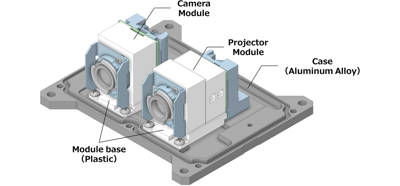
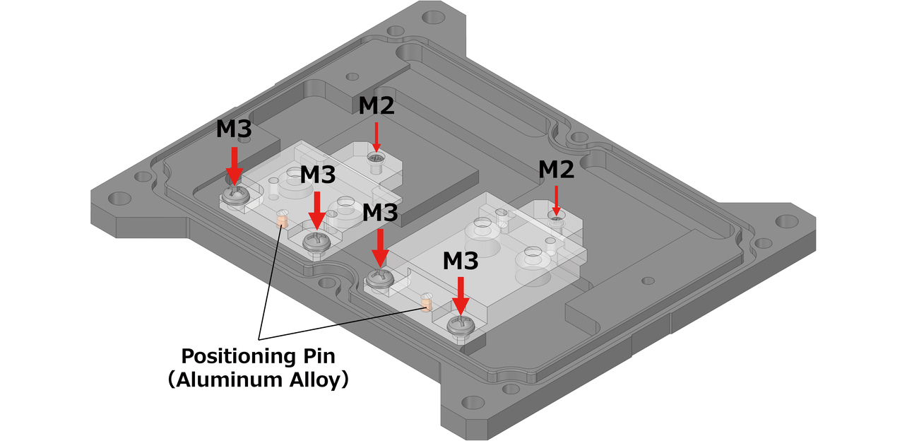
The 3D vision sensor projects a pattern onto an object to obtain and analyze image information thereby identifying the correspondence between the projector (light projection) and camera (light reception) modules shown in Fig. 2 to calculate the measured distance value3). If estimated based on the distance measurement principle and the required product accuracy, even structural variations on the micrometer (μm) order will affect the sensing characteristics on the order of several millimeters. Expansion and shrinkage due to ambient temperature changes cause particularly significant impacts on accuracy. Hence, we adopted the resin-to-aluminum alloy bolted joints shown in Fig. 3 to safeguard the stability of distance measurement accuracy from sudden and significant temperature fluctuations, such as those caused by heat shock. In addition, we adopted a structure with positioning pins provided on the enclosure side to improve the positioning accuracy of the modules used.
However, in an evaluation assuming heat shock (hereinafter “thermal shock test”), the measured distance value varied beyond the tolerance in the initial cycle, giving rise to the need for immediate countermeasures. We inspected the product for its post-test condition in preparation for a causal analysis. The inspection found that the M2 screws for fastening the resin and aluminum alloy had become loosened, albeit only to a level unproblematic for module fixation per se. It is generally known that dissimilar material fastening easily decreases in fastening performance under heat load. Preceding studies confirmed, both by actual measurement and analysis, that under cyclic heat loading, dissimilar material bolted joints become loosened more easily than bolted joints composed of a single material4,5). Therefore, for 3D vision sensors and other devices with structural components whose infinitesimal deformations or geometric configuration affects the output characteristics, dissimilar material fastening will probably become the affecting factor during temperature changes.
However, even under the same sample and conditions, the variation amount in the measured distance value was observed to vary significantly and could not be reproducibly evaluated. As a result, the obtained verification results were unsatisfactory, leaving unanswered questions such as how the loosening affected the measured distance value or whether the measured distance value was affected by factors other than the loosening.
2.2 Change in fastening force under heat load
The first thing to do toward clarifying the behavior of the variation of the measured distance value was to understand how the identified screw loosening had happened. Factors probably responsible for the loosening under heat load included slippery contact surfaces (threaded portion, bearing surface portion, and fastened object surfaces) due to reduced fastening force. Hence, we used a simple mechanical model to represent the fastened state under heat load and estimate its tendency.
Let us start with Coulomb’s friction law, which is the equation known to describe the state of a contact surface. Theoretically, in Coulomb’s friction, a static friction force occurs equal to and opposite in direction to the acting force, whereby the equilibrium (or stasis) of forces is maintained. Moreover, when the acting force exceeds a threshold, the contact surface transitions to a slip state with a certain degree of dynamic frictional force. Let the force per unit area under transition to a slip state be the limiting static frictional stress σlim, which is given as Eq. (1):

where μ is the static friction coefficient of the contact surface, P+ΔP is the contact pressure at each point in time, P is the contact pressure under normal temperature conditions, and ΔP is the contact pressure increment due to temperature change. One can estimate that in a bolted joint, P and ΔP, by definition, are in proportional relation to FB and ΔFB, the axial force occurring in the screw and its increment value, respectively. Accordingly, unless loosening occurs during assembly (under normal temperature conditions), ΔFB plays a critical role in determining the friction condition. Here, Fig. 4 shows the configuration of the dissimilar material bolted joints in the 3D vision sensor as an example to consider a fastened state in the real world. From the physical property value of each member, the relationship among the linear expansion coefficients for Material-I, Material-II, and the screw, α1, α2, and αB is given as α1 ≫ α2, αB. FB, the axial force in the screw, occurs under tightening torque during assembly. With a temperature change added under these conditions, each member starts to expand thermally according to its dimensions/physical properties. However, each member differs in thermal expansion amount from the others and prevents the others from free thermal expansion thereby causing ΔFB.
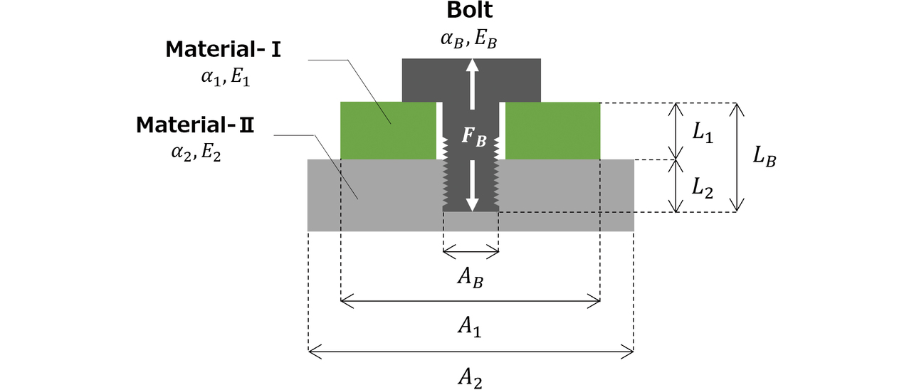
Fig. 5 shows a simplified mechanical model of the dissimilar material bolted joint to estimate the ΔFB caused by differing amounts of thermal expansion. When considered with respect to the axial direction of the screw, each member should supposedly expand by the amount shown in Fig. 5. However, the bearing surface prevents the expansions whereby the equilibrium of forces is reached with the sum of the displacement amounts of Material-I and Material-II agreeing with the displacement amount of the screw. At this point, thermal stress-induced ΔFB occurs to the screw according to the temperature change amount ΔT. ΔFB can be approximated as in Eqs. (2) and (3) by solving the equation of equilibrium in the axial direction:


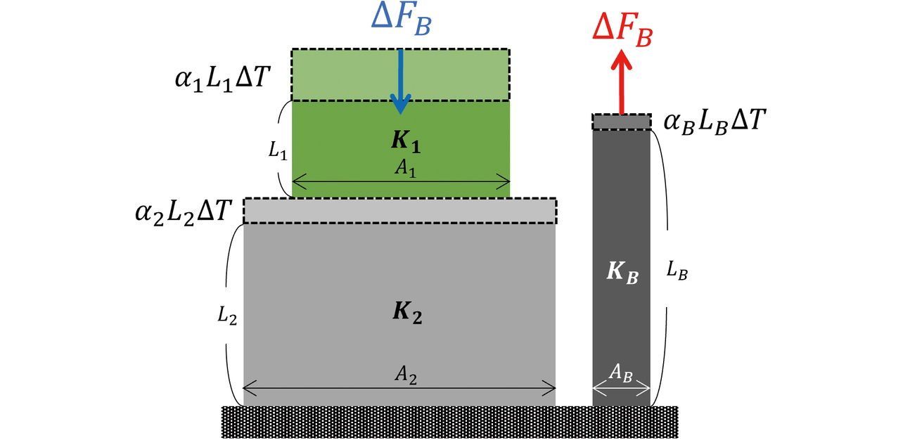
In Eq. (2), Ki (i = 1, 2, B) denotes the axial stiffness of Material I, Material II, and the screw. This value replaces Ei Ai/Li, where Ei is the Young’s modulus of Material i, Ai is the cross-sectional area of Material i, and Li is the member length of Material i. From Eq. (2), ΔFB takes a negative value under low temperatures, reducing the screw’s axial force and contact pressure.
On the other hand, shearing stress occurs on each contact surface and serves as the primary factor responsible for the slip-inducing force. Similarly to the case with ΔFB, this shearing stress increases or decreases as affected by differing amounts of thermal expansion. Its value is proportional not to ΔT but to |ΔT|, the absolute amount of any temperature change. Accordingly, one can make an educated guess that on the lower-temperature side, where a drop in σlim and an increase in shearing stress occur simultaneously because of a decrease in ΔFB, a condition occurs that can easily lead to a slippery contact surface or a loosened screw, contributing to the variation of the measured distance value.
3. Dissimilar material bolted joint’ behavior reproduction using FEM analysis
3.1 Analysis model creation
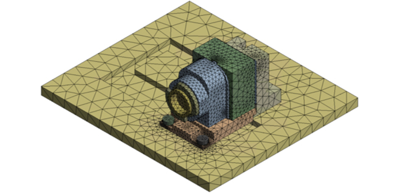
This section presents and explains an analysis model able to reproduce the phenomenon at issue, a model necessary for verification regardless of the forward-problem and inverse-problem approaches. To reproduce the thermal shock-induced behavior of the bolted joints, we performed a thermal stress analysis considering the nonlinear contact conditions. For the convenience of geometric model creation, we omitted parts irrelevant to optical parts fixation and simplified geometric details. Of the two optical modules, we only analyzed the projector-side module, which accounted for most of the influence on the variation of the measured distance value. Fig. 6 shows the mesh-split model created.
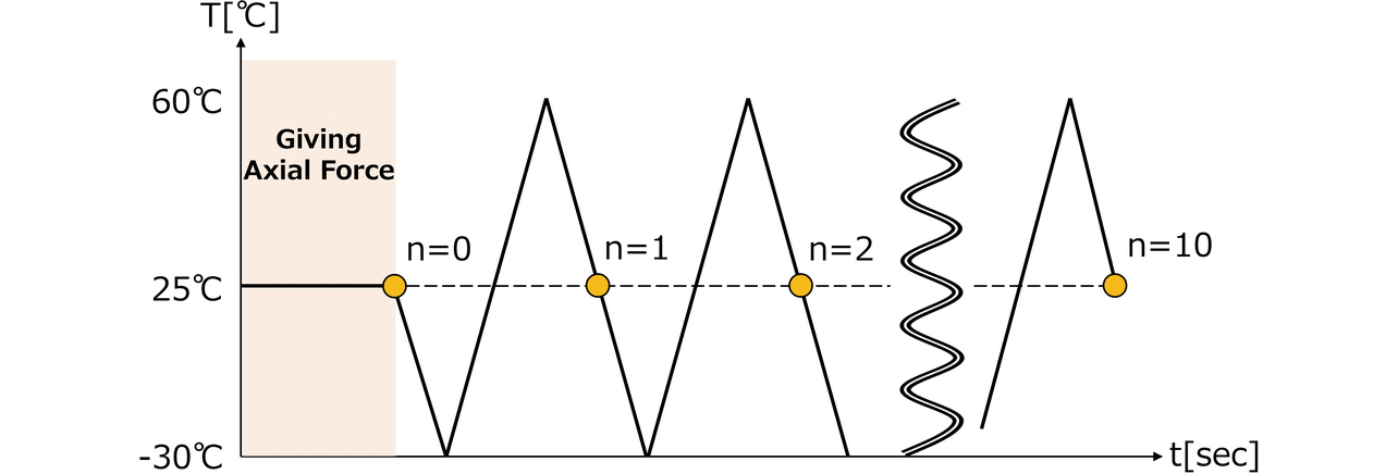
Next, let us move on to the boundary conditions. To simulate a thermal shock test, we applied an axial force to each screw at the reference temperature as shown in Fig. 7. Following the application of the axial force, we added the temperature history of the same ten cycles as under the test conditions. The relationship between FB and the tightening torque value Tq is expressed as in Eqs. (4) and (5) based on the dimensions and friction coefficient of the screws:6,7)


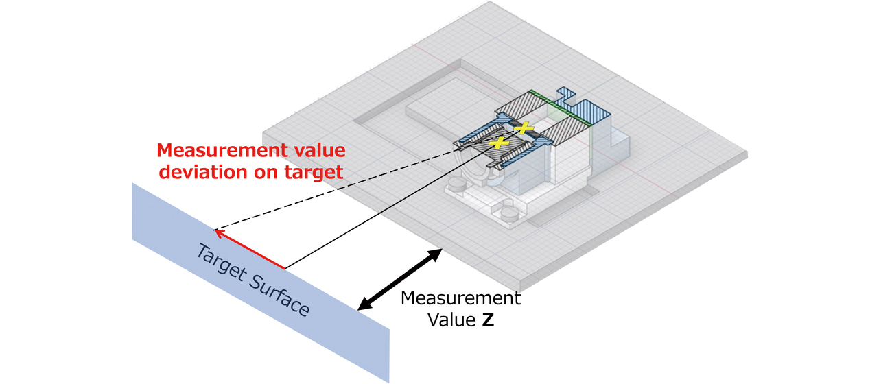
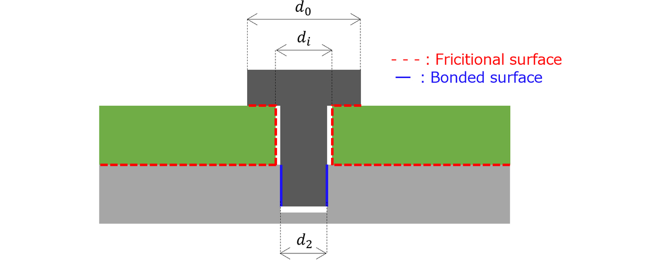
In Eq. (4), μ1 and μ2 are the friction coefficients on the bearing surface and the thread, respectively. Meanwhile, β, γ, d2, and dw are the four screw dimensional parameters, in other words, the thread lead angle, the thread ridge angle, the effective thread diameter, and the equivalent friction diameter of the bearing surface. Eq. (5) derives the equivalent diameter of the bearing surface and can be obtained from the outer diameter d0 and inner diameter di of the contact area of the screw’s bearing surface. We determined the axial forces of the M2 and M3 screws as 339 N and 713 N, respectively, by substituting the tightening torque value, screw dimensions, and friction coefficient into the above equations. Note that ΔZ, the variation amount of the sensor-measured distance value, resulted from the deviation on the target due to the change in the geometric positional relationship between the optical parts as shown in Fig. 8. Therefore, the displacement amount per cycle obtained for each optical part was converted into the amount of deviation on the target. From this deviation amount and the respective optical parameters, ΔZ was calculated.
Let us end this subsection by explaining contact modeling. To prevent the deterioration of convergence for the bolted joint and the excessive expansion of the model size, we avoided reproducing the geometric details of the thread portion and, as shown in Fig. 9, rendered only the thread-equivalent portion as a glued surface and all the other contact surfaces as Coulomb’s friction surfaces. As our contact algorithm, we used the augmented Lagrange method to balance convergence and accuracy. For the modeling and analysis mentioned above, we used AYSYS Workbench Mechanical 2021R2.
3.2 Validation of the analysis results and the model
Fig. 10 shows the absolute values of the variation amount of the sensor-measured distance value, |ΔZ|, obtained by measurement and FEM analysis. The analysis captured the tendency of the absolute value |ΔZ| to become large in the first cycle, as observed commonly across the sample during actual measurement. On the other hand, one should note that analyses tend to underestimate more than measurements. Responsible factors likely include failure to factor in parts’ temperature distributions or temperature dependencies of various physical properties, overestimation of the stiffness of the threaded portion per glue definition, and errors involved in the conversion formula for the measured distance value.
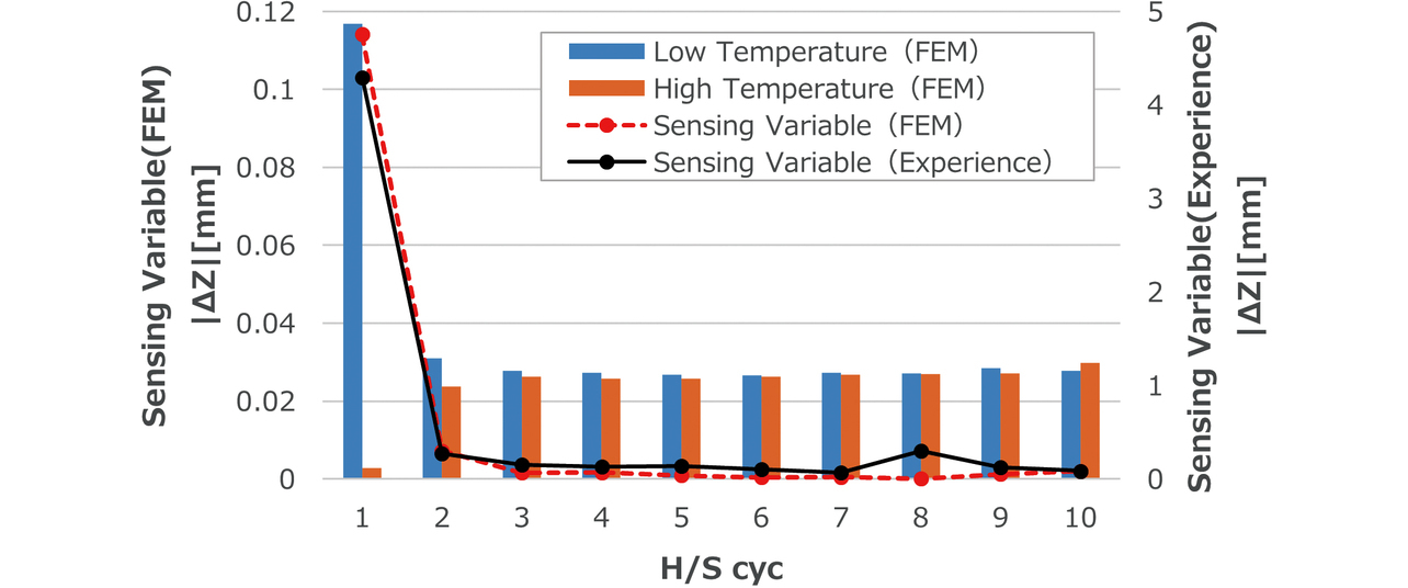
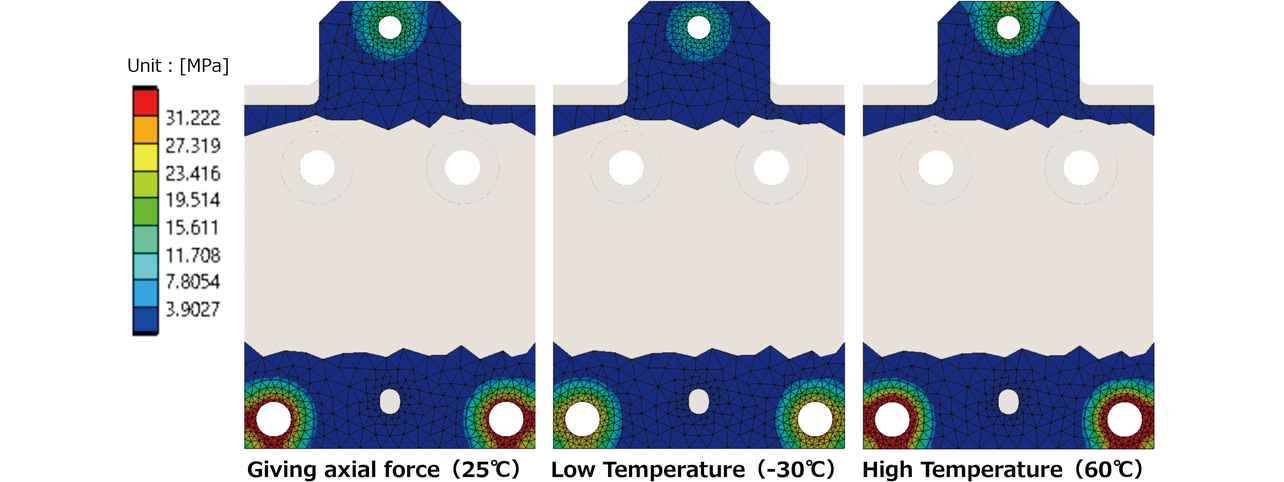
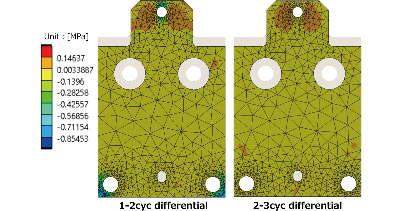
The bars in the bar chart indicate |ΔZ| during the low/high-temperature process in single cycles. In the first cycle, |ΔZ| during the low-temperature process appears dominant. Fig. 11 shows the contact pressure between the resin base and the aluminum alloy-made enclosure. The contact pressure differed depending on the temperature and dropped by approximately 30% under low temperatures from the level under high temperatures. All such differences can be explained as results originating from the decrease in the contact pressure increment ΔP explained in Subsection 2.2. The probable cause of the significant decrease in |ΔZ| from the second cycle onwards was that the shearing stress accumulated from slip occurrences was released. Fig. 12 shows the cycle-to-cycle differences in the maximum shearing stress. The maximum shearing stress around each bolted joint decreased by up to approximately 1 MPa between the first and second cycles but was not observed to drop between the second and third cycles so noticeably as between the first and second cycles. This observation indicates that the shearing force acting during the first cycle decreased from the second cycle onwards.
The change in the qualitative behavior of |ΔZ| or in each physical quantity (contact pressure and shearing stress) during the actual measurement mentioned above agreed with the theory. Hence, we determined it possible to reproduce the tendency of the phenomenon under investigation. The next section considers variations likely to affect the above phenomenon.
4. Verification by inverse-problem approach and FEM analysis
4.1 Specific flow of logic verification
This subsection explains the specific flow of our inverse-problem approach. First, some input values to the analysis model, such as parts dimensions, physical properties, or load conditions, were identified as variables, followed by accumulating analysis results under each condition using the Design of Experiments (DoE). For the present case, what mattered along with contact was the inability to obtain results reproducibly even under the same conditions and sample. Accordingly, we focused on the following two: load conditions and error accumulation during assembly.
First, with regard to the load conditions, the axial force occurring in each screw was allowed to vary. In fastening by a standard torque method, the axial force would be seen to vary, even with the torque value precisely controlled. The JIS states that the ratio of the maximum to the minimum value of axial forces under the same torque (tightening coefficient) should fall within the range from ca. 1.4 to 38). Therefore, in the present case, where infinitesimal displacements/deformations mattered, the axial-force variations should be considered regardless of the thread diameter. However, if the friction coefficients were the variables according to Eqs. (4) and (5), a massive number of parameters would result. Another problem would be that the axial force of each screw cannot be handled independently. Therefore, the axial forces of the M2 and M3 screws fixing the resin base to the aluminum alloy-made enclosure, as shown in Fig. 13, were the direct variables.
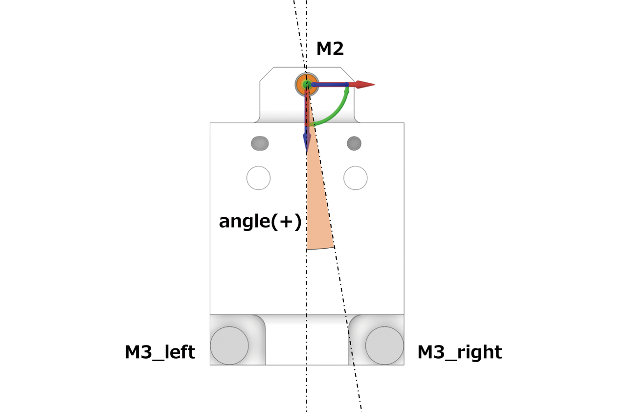
Next, for the error accumulation during assembly, the mounting position of the resin base was allowed to vary. Preceding studies report that various tolerances of screws and fastened objects also significantly affect fastening performance9-11). The mounting position of the resin base was defined as the rotational deviation amount/angle of the resin base relative to the axis of rotation around the M2 screw in Fig. 13. The reason is that with the angle varying, the fixed structures (each screw bearing surface and positioning pin) would change their conditions in step with each other thereby enabling more efficient verification than when the variables were the dimensions of each part (resin base, positioning pin, and screw) one by one.
Given that the first cycle was important and dominant in the measurement and analysis, we used the first-cycle ΔZ as the response variable. Table 1 shows the variables and ranges we set. For the Design of Experiments (DoE), we used Latin Hypercube Sampling, which allows users to specify the number of runs and uniformly search the design space. The total sample size was 250 with 80% for the learning of response surface generation and the remaining 20% for accuracy evaluation. For the automatic updating/analysis execution of explanatory variables defined on the analysis model and for the detailed DoE setting, we used modeFRONTIER 2022R3.
| Variable | Category | Range |
|---|---|---|
| M3_right | Explanatory variables | 374 N to 713 N |
| M3_left | Explanatory variables | 374 N to 713 N |
| M2 | Explanatory variables | 180 N to 339 N |
| angle | Explanatory variables | −0.29° to 0.29° |
| ΔZ | Response variables | \ |
After the completion of sample acquisition by analysis and DoE, methods, such as the tendency visualization or contribution analysis, were used to select the evaluation conditions of interest or characteristic areas. However, at this point, the analysis results should be handled as a mere numerical data group and examined without adding physical interpretations. Finally, the analysis results were checked for each evaluation condition selected, and physical interpretations were added to estimate an appropriate form of logic.
4.2 Data acquisition results and logic estimation/verification
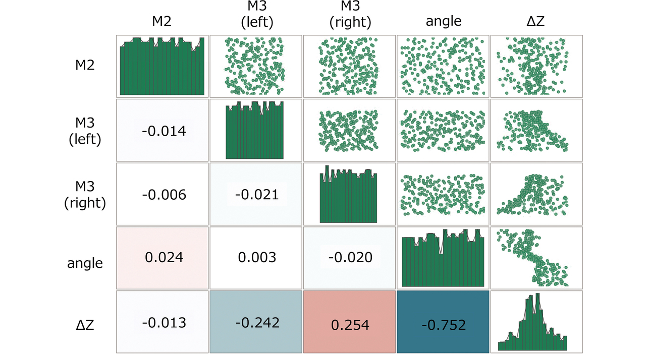
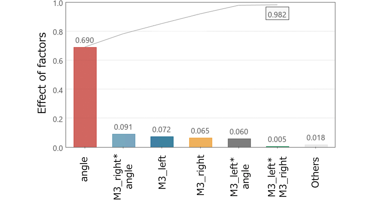
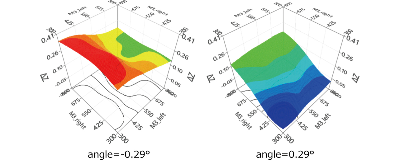
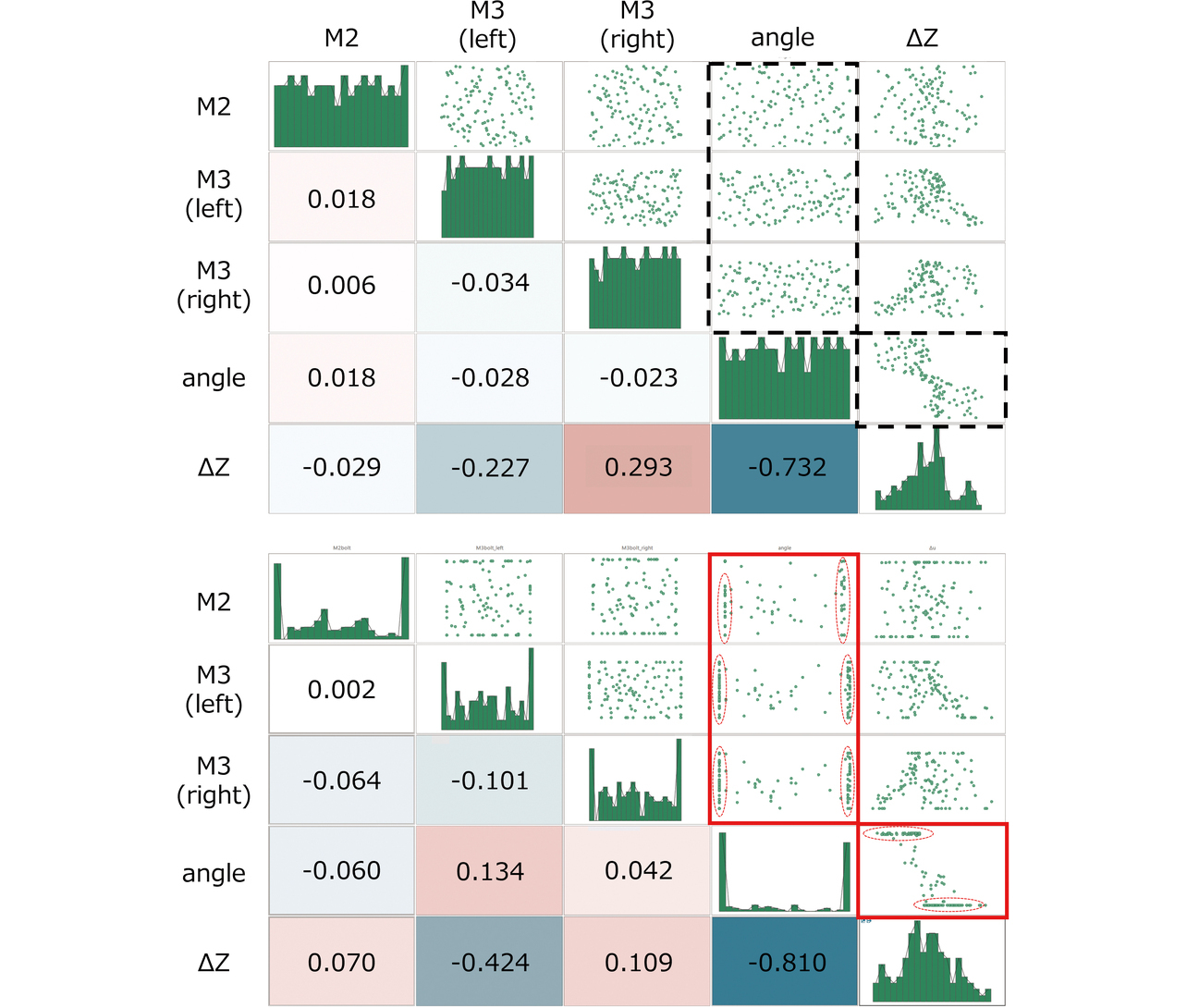
Figs. 14 and 15 show the sampling and contribution analysis results, respectively. The variable angle showed the highest correlation coefficient and contribution, while M2 showed the lowest. Moreover, M3_right and M3_left showed similar correlation coefficient and contribution values. The scatter plots for these two variables show that their tendencies are symmetrical horizontally. Fig. 16 shows the response surfaces created for detailed visualization of their tendencies. We used a radial basis function (RBF) with a coefficient of determination R2 of 0.95, higher than achievable with any other method compared, for surface generation by interpolation between sampling points. The response surfaces with the “angle” = 0.29° and −0.29° revealed that “angle” was the factor that governed the direction of ΔZ. Besides, we confirmed that “M3_right” was the significant factor where “angle” > 0 and “M3_left” where “angle” < 0.
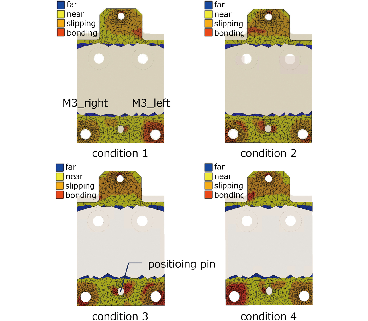
Based on the analysis results, we performed recalculations for the four conditions shown in Table 2: two conditions with ΔZ having a large absolute value and another two conditions with M3_right and M3_left swapping their values. Fig. 17 shows the distribution of the contact state between the resin base and the enclosure under each condition (one should note that these distributions are shown as bottom views and horizontally inverted). Let us first compare the distributions of contact state for Conditions 1 and 2 with M3_right and M3_left swapping their values when “angle” = 0.29°. Under Condition 1, M3_right was low at 374 N whereby the surrounding area was all in a slip state. Meanwhile, under Condition 2, the area around M3_left remained in a glued state. Then, with “angle” = −0.29°, whereas the area around M3_left was all in a slip state under Condition 4, the area around M3_right remained in a glued state under Condition 3, exhibiting a behavior completely opposite to that with “angle” = 0.29°. Our theoretical guess is that a reduced axial force led to an increased slip risk, whereby a singular phenomenon occurred under Conditions 2 and 3, respectively. Fig. 17 also shows an event unique to Conditions 2 and 3, in other words, a highly glued state in the area around the positioning pin.
| Variable | Condition 1 | Condition 2 | Condition 3 | Condition 4 |
|---|---|---|---|---|
| M3_right | 374 N | 713 N | 374 N | 713 N |
| M3_left | 713 N | 374 N | 713 N | 374 N |
| M2 | 180 N | 180 N | 180 N | 180 N |
| angle | 0.29° | 0.29° | −0.29° | −0.29° |
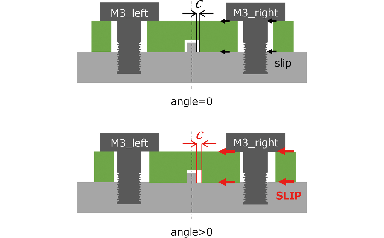
The probable factor responsible for the occurrence of the above behavior was the clearance of the positioning pin part. Fig. 18 shows the configuration of the front-side portion of the resin base. When “angle” > 0 due to assembly variations, a difference in the amount of clearance occurred between the right and left sides of the positioning pin part, as shown in Fig. 18. With “angle” > 0 and M3_right low at 374 N (Condition 1), it follows from the theory and analysis results that under low temperatures, the area around the left-side M3 screw was in a glued state while the area around the right-side M3 screw was in a slip state. Therefore, the resin base around the right-side M3 screw showed a right-to-left slip behavior. In this case, with “angle” > 0, the large amount of clearance c for the slip direction increased the allowable slippage, probably whereby a deviation also occurred in the modules and optical parts therein before and after the temperature change, resulting in a large ΔZ. On the other hand, with “angle” > 0 and M3_left low at 374 N (Condition 2), the amount of c probably became extremely small, resulting in a small ΔZ. A similar behavior explains Conditions 3 and 4, under which the correspondence between c and the value of the axial force in the screw was the simple inverse of that under Conditions 1 and 2.
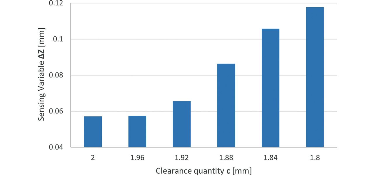
We examined the change in ΔZ with c changed under Condition 2 to validate the above hypothesis. More specifically, the positioning pin’s outer diameter D (reference dimension = 2 mm) was gradually reduced in increments of 0.02 mm to increase c. Fig. 19 shows the results obtained. It turned out that, even under Condition 2, ΔZ increased with the decrease in D (increase in c). Therefore, the conclusion is that, depending on the increase/ decrease in c during assembly, the slippage in the resin base varied, affecting ΔZ.
From the observations made so far, the factors ultimately found responsible for the increase in ΔZ are the following two:
- Amount of clearance c of the positioning component for the slip direction
- Interaction between the amount of clearance c and the axial force in the M3 screw
Meanwhile, either of the following conditions can reduce ΔZ:
- Reduction/optimization of the amount of clearance c
- Enhancement of the axial force in the M3 screws or all screws
However, the value c cannot be directly measured because of the product structure and can easily vary depending on the dimensional tolerances and the assembly procedures for the individual parts. Moreover, the axial force in each screw with a small outer diameter is hard to measure with an instrument, such as an ultrasonic axial force meter or a strain gauge. These axial forces can vary depending on the surface condition or various dimensions as shown by Eq. (4), and their variations are unstable similarly to those of c. Therefore, the challenge toward ΔZ reduction would be a solution from the design perspective, such as changing the positioning design or the optical modules’ materials, rather than those from the production process perspective.
4.3 Efficiency enhancement of our inverse-problem approach
Experimental design, which constitutes the core of an inverse-problem approach, is seriously challenged by the trade-off relation between the number of available runs (or the amount of available time) and accuracy. Considering exploiting this approach in the design process with the limited time or person-hours available for verification, one would hope to achieve accuracy with the minimum sample size and obtain the maximum amount of useful information. Moreover, a faster verification cycle per run would make it possible to change/add parameters, for example, for additional verification or to compare multiple structure proposals, leading to a more fulfilling design. However, it is challenging to predefine an appropriate sample size or DoE method for an unknown design space. To do so can lead to problems, such as increased person-hours due to excessive sampling or reduced accuracy due to an insufficient sample size.
For the present case, we considered adaptive DoE as a method to solve such problems. An adaptive DoE method internally repeats the cycles of sample acquisition and design space evaluation without a predetermined sample acquisition plan. As such, the procedure is expected to improve accuracy with a small sample size12,13). In the present study, we focused on Multivariate Adaptive Cross-validating Kriging (MACK)14), a type of adaptive DoE. MACK is a technique that first performs coarse sampling within the design space, then internal cross-validation of the response surface, and finally, resampling of high-uncertainty areas. For this paper, we compared MACK with Latin Hypercube Sampling to verify the effectiveness of its use.
Fig. 20 shows the sampling results for each method. The design space sampling results obtained by Latin Hypercube Sampling show a uniform distribution. By contrast, the results obtained by MACK exhibit a biased distribution. The areas near the upper and lower limits of the “angle” determined in Subsection 4.2 as having a high contribution were particularly intensively sampled, which led to an educated guess that areas prone to ΔZ variations were intensively explored. The application of MACK reduced the sample size required to achieve target accuracy from 100 to 40 items. This reduction in sample size compares with that in computation time from around 25 to 10 hours. The above results confirm that MACK can efficiently search for characteristic areas in a design space and significantly contribute to reducing the required period for verification based on an inverse-problem approach.
5. Conclusions
For a problem that involves uncontrollable/unobservable variations during experimental evaluation and makes the product characteristic behavior difficult to elucidate, we turned our attention to a method that uses both FEM analysis and an inverse-problem approach. This paper was concerned with the variation of the measured distance value obtained by a 3D vision sensor under thermal shock testing. We investigated this variation using the method mentioned above. As a result, the following logic emerged with clarity: the loosening of the M2 screws detected in the actual device did not contribute to the variation of the measured distance value, and the affecting factor was the amount of clearance of the positioning pin for the slip direction of the resin base during the decrease of axial force in M3 screws. Moreover, adopting MACK as our DoE method for sampling efficiency enhancement, we reduced the sample size N by up to around 60% in the present case thereby demonstrating that MACK is an effective method for efficiency enhancement.
Where multiple variations affect the results, the challenge is to estimate an appropriate form of logic and set an appropriate set of evaluation conditions, causing extreme difficulty in logic verification based on the forward-problem approach. In this study, we tackled such a challenge using an inverse-problem approach, thereby demonstrating that the inverse-problem approach is effective in problem-solving and allows the designer to perform logic verification with limited person-hours and without repeating trial and error to no avail. These technical achievements can be applied to various technical challenges, leading to shorter development lead times and faster product launch cycles.
Future challenges include improving accuracy and efficiency. First, one of the challenges from the accuracy perspective is to improve the accuracy of thermal stress analysis with consideration given to the detailed physical properties of the resin base. Resins are more significantly affected by temperature dependency or molding process-induced anisotropy than metal materials and are considered likely to be significantly affected by rapid temperature fluctuations. As such, resins should be subjected to various tests, including thermomechanical analysis (TMA), to obtain detailed physical property values and incorporate them into the analysis. On the other hand, one of the challenges from the efficiency perspective is automatic sample size determination. For the present case, the author specified the sample size beforehand and obtained a sample to examine the effectiveness of MACK. However, the sample size should not be predetermined by the user in the first place, and sampling should preferably be terminated when a certain level of accuracy is reached. Therefore, the concept of achieving the intended accuracy and a specific method therefor must be developed using the maximum number of available runs as the only constraint.
Moving forward, we will continue with the above efforts to achieve more accurate thermal stress analysis and more efficient sampling for a further improved ability to analyze occurrence events or product behaviors with a view to developing a design technology able to create highly robust designs.
References
- 1)
- M. Ikeda, “Innovation of the Method for Balancing Trade-off Requirements in Product Design Process,” (in Japanese), OMRON TECHNICS, vol. 52, no. 1, pp. 105-110, 2020.
- 2)
- K. Sato et al., “Feasibility Study about Design Process of Power Electronics Converters by Optimization Method Applied Machine Learning,” (in Japanese), OMRON TECHNICS, vol. 54, no. 1, pp. 101-106, 2022.
- 3)
- J. Ota et al., “A Small and Light 3D Vision Sensor for Robot Arms with Robustness in Factory Automation,” (in Japanese), OMRON TECHNICS, vol. 54, no. 1, pp. 60-65, 2022.
- 4)
- T. Sawa et al., “Mechanism of Rotational Screw Thread Loosening in Bolted Joints under Repeated Temperature Changes,” (in Japanese), in Proc. Yamanashi Conf. (JSME), 2007, pp. 149-150.
- 5)
- M. Kobayashi et al., “Influence of the Tightened Material on the Axis Force Behavior of Bolted Joints with Heat Load,” (in Japanese), in Proc. Autumn Conf. Tohoku Branch, JSME, 2016, vol. 52.
- 6)
- S. Hareyama, “A Study on Bolt Axial Tension Control by the Calibrated Wrench Method (1st Report, Distribution of Bolt Axial Tension),” (in Japanese), Trans. Jpn. Soc. Mech. Eng., Ser. C, vol. 53, no. 495, pp. 2373-2379, 1987.
- 7)
- M. Kobayashi, “Basic Knowledge of the Bolted Joints,” (in Japanese), J. Jpn. Soc. Precis. Eng., vol. 81, no. 7, pp. 619-622, 2015.
- 8)
- Japanese Industrial Standard, JIS B 1083, 2008.
- 9)
- M. Okada et al., “A Study on Bearing Surface Pressure Distribution of Bolted Joints (Influences of Angular Deviation of Bearing Surface),” (in Japanese), Trans. Jpn. Soc. Mech. Eng., Ser. C, vol. 70, no. 699, pp. 3324-3330, 2004.
- 10)
- T. Fukuoka et al., “Improvement of Tightening Accuracy of Torque Control Method by Taking into Account Geometric Errors in Threaded Fasteners,” (in Japanese), J. JIME, vol. 51, no. 2, pp. 238-245, 2016.
- 11)
- M. Kasai et al., “Effects of Accuracy of the Nut Bearing Surface on Tightening Condition of Hollow-Type Bolted Joint: 1st Report, Relationship between Accuracy of the Nut Bearing Surface and Strain Distribution in the Axial Direction of Hollow-type Bolt,” (in Japanese), Trans. Jpn. Soc. Mech. Eng., Ser. C, vol. 61, no. 583, pp. 1136-1142, 1995.
- 12)
- T. Ueno et al., “Efficiency Improvement of X-Ray Spectroscopy Experiment by Machine Learning,” (in Japanese), Vac. Surf. Sci., vol. 62, no. 3, pp. 147-152, 2019.
- 13)
- K. Shimoyama et al., “A Kriging-Based Dynamic Adaptive Sampling Method for Uncertainty Quantification,,” Trans. J. Soc. Aeronaut. Space Sci., vol. 62, no. 3, pp. 137-150, 2019.
- 14)
- ESTECO S.p.A. “modeFRONTIER.” https://engineering.esteco.com/modefrontier/ (Accessed: Oct. 1, 2023)
The names of products in the text may be the trademarks of each company.