


Improving Direction Estimation Accuracy of Millimeter-wave Radar by Suppressing Unnecessary Radiation from Transmission Lines
- Millimeter-wave Radar
- Estimating Direction-of-arrival
- Waveguide
- SIW
- Suppressing Unnecessary Radiation
Millimeter-wave radars have been drawing interest as a means of contactless sensing of the positions of people and objects and are expected to be used in a wide range of fields, such as automotive, transportation infrastructure, factory automation (FA), and healthcare. In order for radars to correctly detect the position of the targets, it is necessary to estimate the direction of arrival of the radio waves with high accuracy. When radio waves are radiated from parts other than the antennas, such as transmission lines, the accuracy of estimating the direction of arrival decreases. Therefore, we introduce substrate-integrated waveguides (SIWs) in which the electromagnetic field propagates inside the substrate layer instead of the conventional transmission line formed on the surface of the substrate. Then, we investigated the suppression of unnecessary radiation and the improvement of the accuracy of the direction-of-arrival of radio waves. In this paper, we use electromagnetic field simulations to show the effect of suppressing unwanted radiation and show that the error in the direction-of-arrival estimation is improved from the conventional 4.1° to 1.2°. This result is effective in providing millimeter-wave sensing that detects the position of the targets with high accuracy.
1. Introduction
In recent years, studies have been underway on the application of radar technologies to contactless methods of human and object detection. Radars can detect the target’s position and velocity regardless of environmental conditions, such as backlight, darkness, or fog. Additionally, radars have advantages in sensing, such as the ease of ensuring privacy. Radars that use millimeter waves (hereinafter “millimeter-wave radars”), in particular, provide high spatial resolutions due to their use of shorter wavelengths (several millimeters) and the broader frequency bandwidths available to them compared to widely used conventional radars. Moreover, advancements in semiconductor production technology have led to lower pricing of millimeter-wave ICs. Furthermore, legal amendments have deregulated millimeter-wave bands. Thus, a favorable environment is emerging for using millimeter-wave radars. Under these circumstances, millimeter-wave radars are expected to find extensive applications in various fields1,2), such as obstacle detection for self-driving cars or autonomous mobile robots (AMR), traffic conditions monitoring (including pedestrians)3), and human health condition monitoring in homes or facilities.
The effective use of millimeter-wave radars for such purposes relies on high-accuracy target position detection. One example is a system consisting of millimeter-wave radars installed near intersections to monitor traffic conditions and to provide detection results to nearby vehicles, thus preventing traffic accidents. This system is required to accurately detect the accurate positions of people and vehicles apart by several to ten-odd meters. An inaccurately detected target’s position can disrupt smooth traffic flow, as may be when a pedestrian is falsely located at a dangerous point at an intersection while the person is actually on a safe sidewalk. Similarly, in a health condition monitoring system, low position detection accuracy can lead to failure to correctly detect the vital signals of multiple individuals close to each other. Let us consider an example of monitoring changes in the health conditions of babies and infants napping in a nursery facility. In this usage scenario, radars installed on the ceiling or walls simultaneously detect the vital signals of multiple babies and infants sleeping close to each other. If position detection accuracy is low in such a case, an individual may be located in a false position that overlaps the point of detection of another individual. In other words, when the radar-received signal is divided into position-specific signals to extract vital signals from the signals corresponding to the points of detection of individuals, overlapping points of detection of multiple persons may lead to the superimposition of these vital signals, giving rise to a concern for the failure to detect vital signals correctly.
Millimeter-wave radar must be able to detect the direction of arrival of radio waves with high accuracy to locate the correct positions. For this purpose, the requirement is that components other than the antenna not emit any radio waves. Among the components of a radar device, one of the likely sources of unwanted radio waves is transmission lines. Typical millimeter-wave radars use an array antenna consisting of antenna elements arranged in an array to estimate the direction of arrival of radio waves without physically turning the antenna. Therefore, to connect spatially separated multiple antenna elements to a single millimeter-wave IC, a transmission line of a certain length must be provided between each antenna element and the millimeter-wave IC. More specifically, in smaller millimeter-wave radars, the antenna, the transmission line, and the millimeter-wave IC are often arranged on a single printed circuit board for the sake of design simplification. Typical transmission lines on printed circuit boards include microstrip lines (MSLs) and grounded coplanar waveguides (GCPWs). MSLs and GCPWs have a relatively low transmission loss on the one hand. On the other hand, however, they are structurally likely to emit electromagnetic fields from their exposed signal conductor to the surrounding space. As a result, they may suffer low direction-of-arrival (DOA) estimation accuracy.
Included among transmission lines with relatively low radio-wave radiation into the air are substrate-integrated waveguides (SIWs). These waveguides are designed to propagate electromagnetic waves to the internal layer of the substrate, which is grounded both front and back. Examples have been reported of configuration designs that use SIWs to supply power to microstrip antennas (MSAs), which are often formed on a substrate4-6). However, these reports have failed to mention the influence of power radiation from the transmission line on the DOA estimation accuracy of radar devices. On the other hand, to determine whether to apply SIWs to a radar device, one must specifically elucidate the benefits of DOA estimation accuracy improvement achievable by introducing SIWs. Accordingly, we performed an electromagnetic field simulation to quantitatively demonstrate the effects of DOA estimation accuracy improvement achievable by introducing SIWs as the power supply lines to MSAs. However, no established DOA estimation accuracy evaluation metrics were available for use in this process. Then, we introduced an evaluation method based on the worst value of estimation errors obtained by sweeping the true direction of arrival in a certain angle range. We confirmed the effectiveness of this method, the details of which will be presented later herein.
First, Section 2 compares the characteristics of SIW, MSL, and GCPW transmission lines. Section 3 presents the electromagnetic field simulation conducted to demonstrate that a millimeter-wave radar device with SIW transmission lines exhibits reduced transmission line radiation. Finally, Section 4 discusses the DOA estimation accuracy improvements achieved by applying our DOA estimation algorithm to the radiation patterns obtained from the electromagnetic field simulation.
2. Characteristics of transmission lines
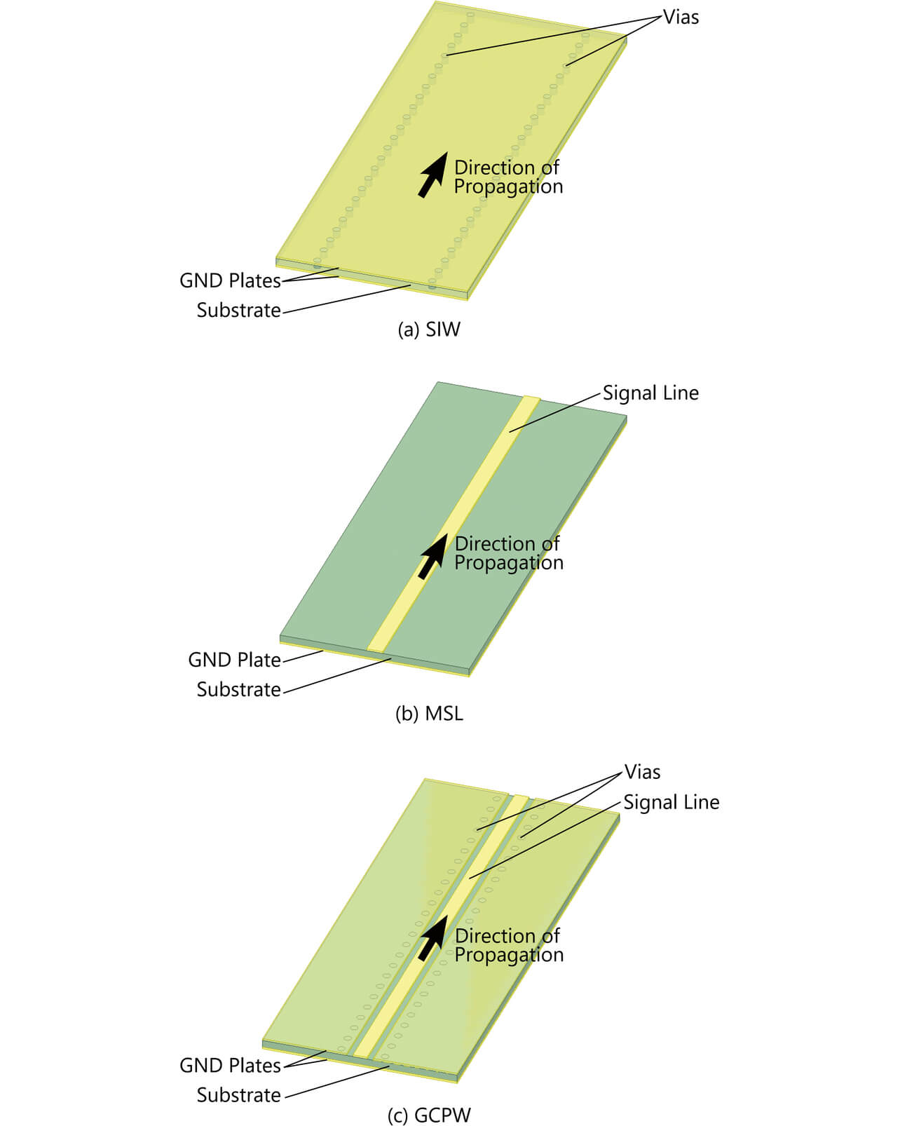
2.1 Design of the SIW
As explained in Section 1, typical millimeter-wave transmission lines formed on substrates include SIWs, MSLs, and GCPWs. Among these options, an SIW transmission line propagates electromagnetic waves between two parallel lines of vias formed on a double-side grounded substrate, as shown in Fig. 1(a). Unlike its MSL and GCPW counterparts shown in Figs. 1(b) and (c), respectively, the SIW transmission line, in principle, has an extremely low level of radiation to space because its design ensures the containment of electromagnetic fields in the substrate. Moreover, this transmission line can be said to be a type of rectangular waveguide because, with its via-to-via spacing being sufficiently close, electromagnetic waves can be regarded as propagating through the area surrounded by metal.
Here, we consider the line width requirement for propagating electromagnetic waves in the 60 to 64 GHz frequency bands used for radars through an SIW. One of the typical characteristics of a rectangular waveguide is the cutoff frequency, which is the lowest frequency for mode-specific propagation. This frequency is given by the following equation:

where c0 is the light speed in vacuum, p and q are mode numbers, μr and εr are the relative permeability and relative permittivity of the medium in the waveguide (i.e., the base material of the substrate), and a and b are the dimensions of the waveguide. In the case of an SIW, a and b can be regarded as the line width and the waveguide thickness, respectively. If the substrate shown in Table 1 is used as an example, b = 0.152 mm, μr = 1.0, and εr = 3.2.
| Item | Value | ||
|---|---|---|---|
| Physical property values | Relative permittivity | εr | 3.2 |
| Relative permeability | μr | 1.0 | |
| Dielectric loss tangent | tanδ | 0.004 | |
| Dimensional values | Substrate thickness | b | 0.152 mm |
| Copper foil thickness | tc | 0.040 mm | |
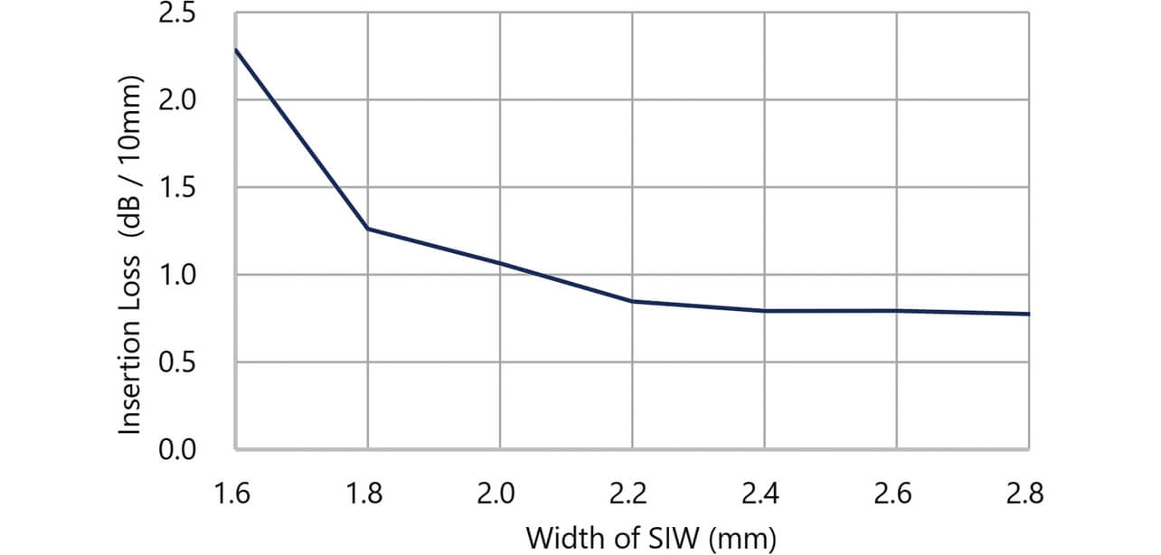
These values show that the line width a must be at least 1.6 mm or more for transmitting TE10 mode with the lowest cutoff frequency. When an electromagnetic field simulation was performed for the insertion loss with the value of a changed for a linear-shaped SIW, the insertion loss showed a decreasing trend until a was increased up to approximately 2.4 mm, beyond which the insertion loss remained almost constant (Fig. 2). As explained in Section 3, if a has a large value, its application to the radar board results in a bend with a small curvature radius, posing the concern of a large loss at the bend. With these points in mind, a was set to 2.4 mm.
Moreover, the via-to-wall spacing was designed to be 0.25 mm or more to allow for cracks that may occur during the production process. Therefore, with a via diameter of 0.15 mm, the via-to-via spacing must be set to 0.4 mm or more, based on which we set the via-to-via spacing in the simulation model to 0.4 mm. Table 2 shows the design values for the line width and the via dimensions.
| SIW | MSL | GCPW | |
|---|---|---|---|
| Line width | 2.400 mm | 0.370 mm | 0.330 mm |
| Via diameter | 0.150 mm | — | 0.150 mm |
| Via-to-via spacing | 0.400 mm | — | 0.400 mm |
2.2 Comparison of the characteristics of waveguides
Subsection 2.2 compares the SIW designed in Subsection 2.1 with its MSL and GCPW counterparts configured to have their signal conductor exposed to the surrounding space for the emissivity to space and the insertion loss at 62 GHz (Fig. 3). This emissivity is defined as follows: a port is provided at each end of the line. Power is supplied from one of the two ports. Some of the input power to the port is radiated from the substrate and released to the outside of the analysis space. The ratio of the power supplied to the port and its portion released to the outside of the analysis space is defined as emissivity.
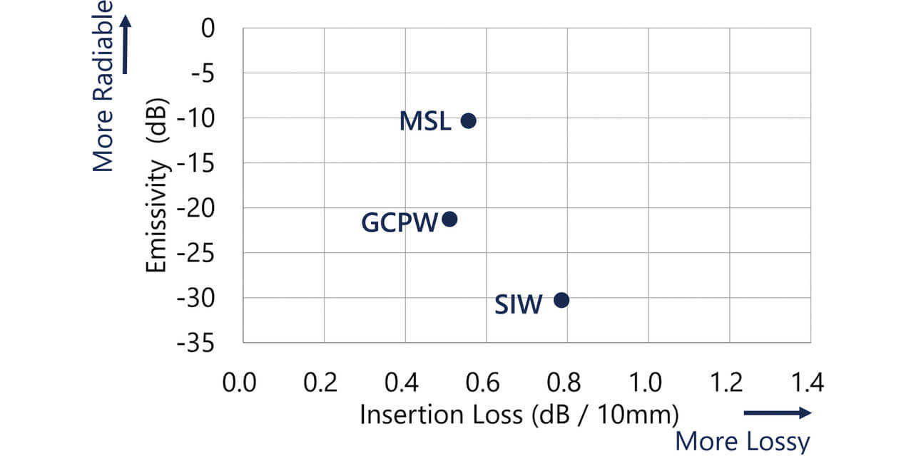
For the comparison, the Ansys HFSS electromagnetic field simulator was used. The GCPW and the SIW were designed to yield a characteristic impedance of 50 Ω. Their specific design values were added to Table 2 above. The substrate length (transmission line length) was set to 10 mm and the substrate width to 4 mm.
Let us first note the emissivity represented by the vertical axis of the graph in Fig. 3. As expected, the SIW showed lower power radiation than the MSL or the GCPW, probably because of its structure in which the area passed through by electromagnetic fields was disposed of between the GNDs on the front and back sides of the substrate, reducing electromagnetic field leakage to the surrounding space.
Let us next turn attention to the insertion loss represented by the horizontal axis of the graph in Fig. 3. The SIW showed a higher insertion loss than the MSL or the GCPW, possibly because, with most of its electric fields contained in the substrate, the SIW had a high dielectric loss, unlike the MSL or the GCPW, which let some of their electric fields pass through the air.
These results show that the SIW is a preferred option to suppress the power radiation from the transmission line as explained above. This option increases the insertion loss but promises to produce the effect of reducing the influence of the power radiation from the transmission line on the antenna radiation pattern.
3. Application of the SIW to the radar board
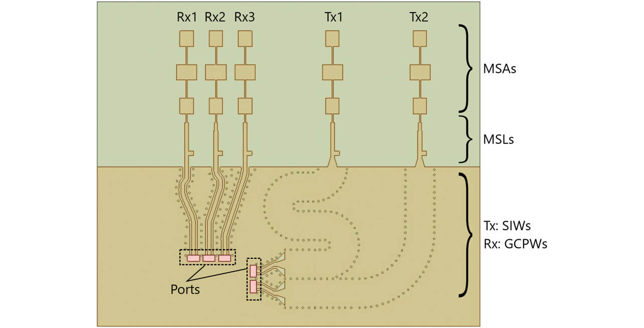
Fig. 4(a) shows the electromagnetic field simulation model that we previously developed for radar boards. In the configuration of this model, two transmitting antennas (Tx1 and Tx2) and three receiving antennas (Rx1, Rx2, and Rx3) were provided on the surface of a substrate parallel to the XY plane, each antenna consisting of three MSAs cascade-connected in the Y-direction to focus beams within the YZ-plane and extended to the GND edge via an MSL-based impedance matching circuit. The wiring from the GND edge to each port (red rectangles in the figure) was provided using a GCPW. The transmission lines to the two transmitting antennas and three receiving antennas were wired to be equal in length. The substrate used was the one shown in Table 1. Considering the proximity between the receiving antennas, the influence of the interconnections was reduced by providing parasitic elements adjacent to Rx1 and Rx3. This model is referred hereinafter to as the “GCPW model,” with which we compared another model equipped with SIW transmission lines instead of GCPW transmission lines.
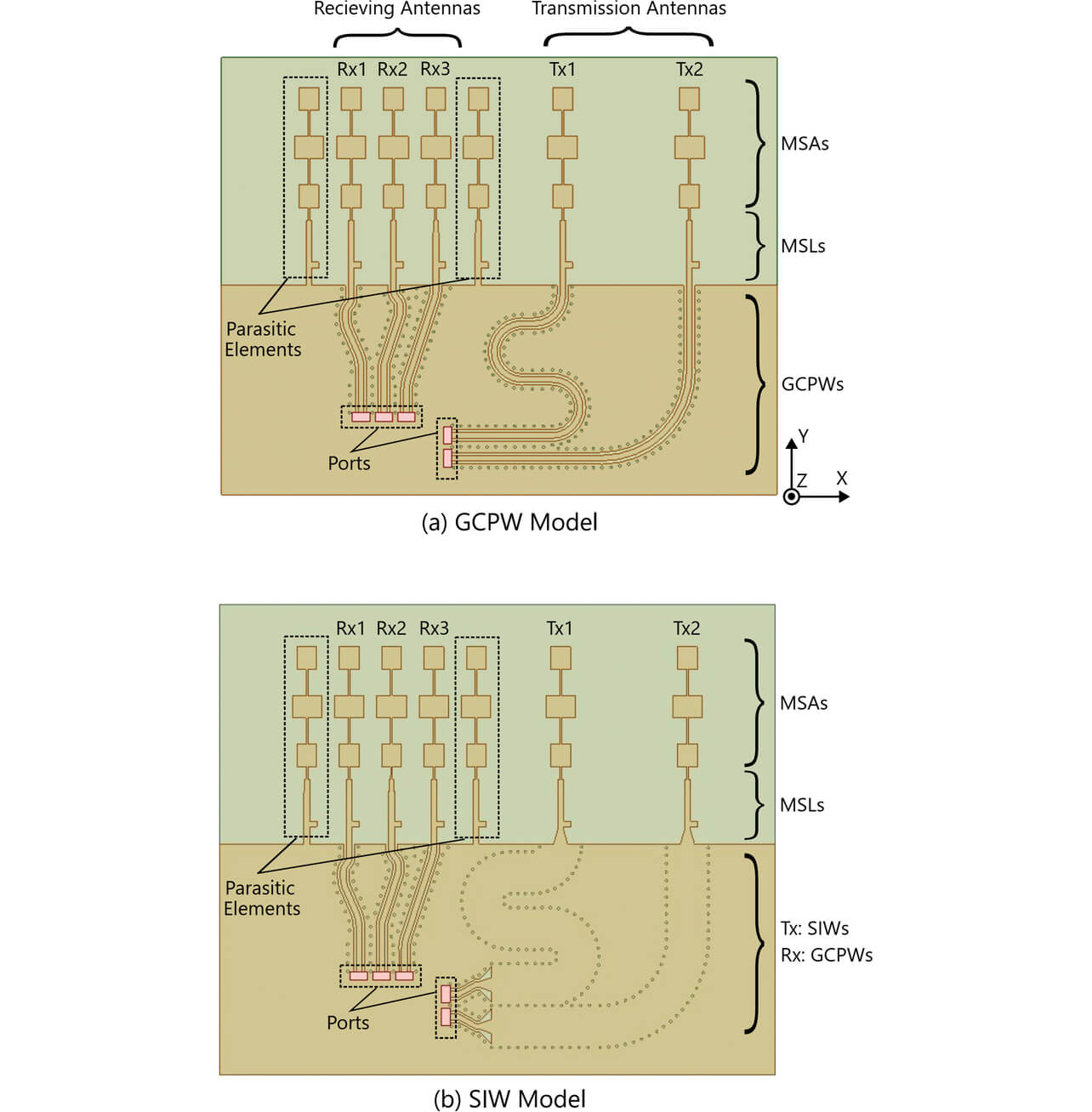
Fig. 4(b) shows the model with its ports and transmitting antennas connected via SIWs instead of GCPWs (hereinafter “SIW model”). In this model, MSLs were connected to SIWs7) at the GND edge and then to ports, near which the SIWs were replaced with GCPWs8). Put differently, the conventional GCPW portions of the transmission lines were mostly replaced with SIWs. As explained above, the MSLs connecting the MSAs to the substrate edge were used for impedance matching and hence were retained without being replaced with SIWs.
Under the premise that the two transmission lines constituting the transmitting system have an equal length, multiple bends must be included in Transmission Line Tx1 with a short straight distance between its port and the antenna. Considering that the port and antenna positions were fixed based on the premise of replacing the transmission lines in the GCPW model, the bends would have a smaller curvature radius with an increasing transmission line width. A smaller bend curvature radius would lead to the concern of an increased transmission loss. Accordingly, based on the consideration results in Section 2, we set the SIW width in the SIW model to 2.4 mm.
4. DOA estimation accuracy improvements
4.1 Radiation patterns
Using the HFSS electromagnetic field simulator, we estimated the radiation patterns of the antennas of the transmitting system and the receiving system of the GCPW and SIW models. In this estimation, we assumed the same amplitude and phase for the input voltages from the ports to the antennas. Figs. 5 and 6, respectively, show the amplitude and phase for the Y-polarized wave radiation pattern of the transmitting system in the ZX-plane at 62 GHz. Here, the azimuth angle in the ZX-plane is defined as 0° for the +Z-direction and +90° for the +X-direction. The graphic representation of radiation patterns for the receiving system is omitted because the GCPW and SIW models had no structural differences in their receiving systems.
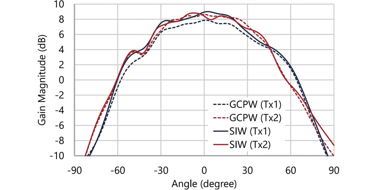
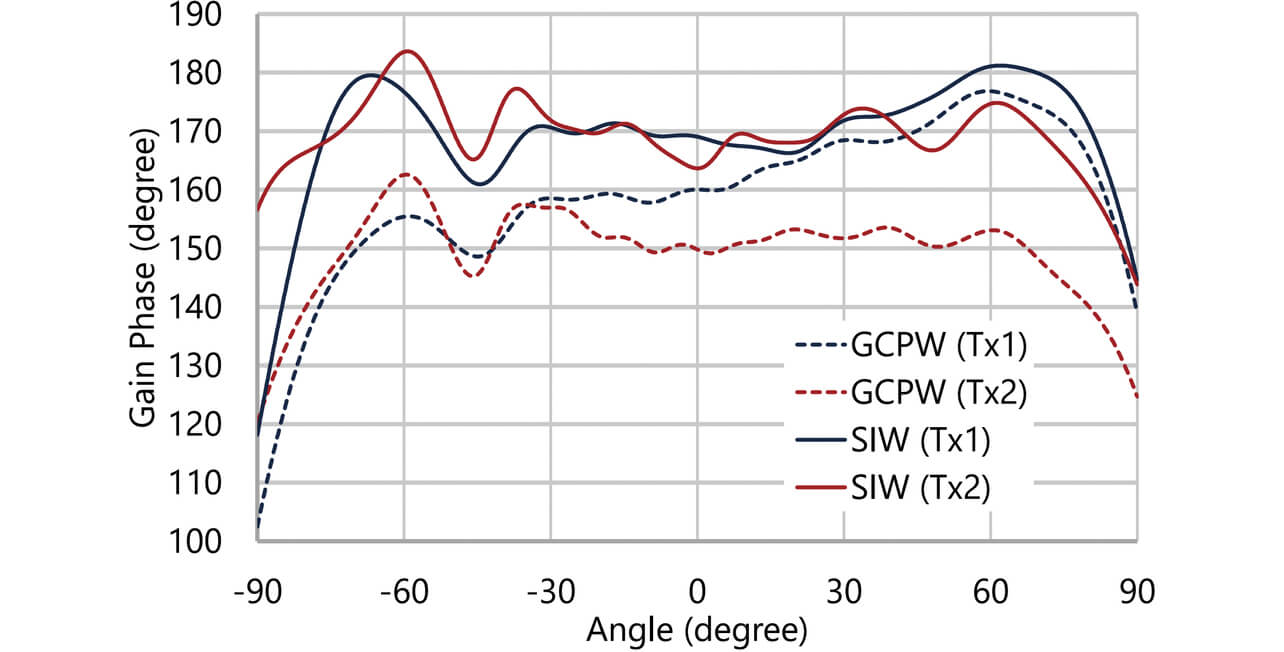
Considering the symmetry of the MSAs about the Y-axis, we expected that the antennas as single elements would show a symmetric directivity with respect to the ZX-plane. It follows then that the closer to symmetry the obtained directivity, the weaker the influence of the transmission line radiation. Figs. 5 and 6 reveal that the SIW model showed directivity closer to symmetry than the GCPW model. This tendency was particularly pronounced in the Tx1 phase patterns of the two models and was also noticeable because the two models were compared for the area around ±45° or ±60° in the Tx1 amplitude pattern. Therefore, we can say that the replacement with SIW transmission lines successfully reduced the influence of the transmission line radiation as intended.
4.2 DOA estimation accuracy calculation method
This subsection describes the method of determining the DOA estimation accuracy. Here, we estimate the direction of arrival by applying the beamformer method, a typical DOA estimation algorithm, to a six-channel MIMO radar consisting of a combination of two transmitting antennas and three receiving antennas provided on a substrate.
When a plane wave simulating a reflected wave arrives from an azimuth θs , the received signal xmn (θs ) to the MIMO channel consisting of the m-th transmitting antenna and the n-th receiving antenna can be expressed as

where Gm (θ ) and Gn (θs ) are the θs -direction gains (complex numbers) of the m-th transmitting antenna and the n-th receiving antenna, respectively, Δφmn is the phase difference caused by the relative positions of the respective virtual array antennas, and A is a coefficient.
When the virtual array mode vector D (θt ) for the azimuth θt is used, Po (θt ), the signal strength in the θt direction, is given as

where [⋅]H is the adjoint matrix of the matrix [⋅] and X (θs )=[x11 (θs ),⋯,xMN (θs )]. It should be noted that M and N represent the number of transmitting and receiving antennas, respectively.
An azimuth spectrum based on the beamformer method can be obtained by calculating Po (θt ) for each azimuth θt . An azimuth that maximizes this azimuth spectrum is the detection azimuth θd .
The above operations allowed us to obtain the radar detection azimuth θd with respect to the true incoming wave azimuth θs . Therefore, the difference between these two azimuths |θd -θs | can be used as the detection error.
On the other hand, no established metric has been available to evaluate the “DOA estimation accuracy for a certain angle range.” Hence, a “DOA estimation accuracy for a certain angle range,” defined as the “angle accuracy guaranteed for that angle range,” can be paraphrased into the “worst value (largest detection error) in that angle range.” In other words, the DOA estimation accuracy s (θl ,θr ) in the angle range [θl ,θr ] is the largest value of |θd -θs | with the true incoming wave azimuth θs moved in the range [θl ,θr ] and can be expressed as

We use this value for DOA estimation accuracy evaluation.
4.3 Verification of DOA estimation accuracy improvements
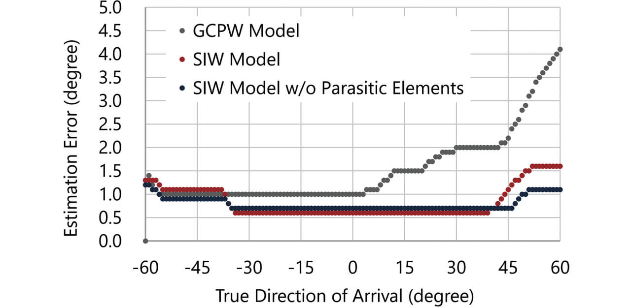
Fig. 7 shows the DOA estimation accuracies calculated based on the results of the electromagnetic field simulation of the gain patterns for the GCPW and SIW models. The vertical axis with respect to the horizontal-axis azimuth θx represents the largest value max (|θd -θs |) of the error resulting from sweeping the true incoming wave azimuth θs from 0° to θx . The sweep angle increment for θx and that for the direction θt , the direction of mode vector generation, were both set to 0.1°. Here, we omitted the correction (calibration) of channel-specific received signals with incoming-wave received signals from the front and other directions.
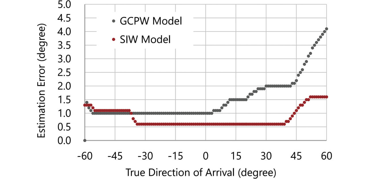
An observation within the range of –60° ≤ θs ≤ 60° finds that the largest estimation error remained at a relatively low value of 1.6° for the SIW model while reaching 4.1° for the GCPW model. In other words, the replacement of the GCPW transmission lines with SIW ones led to an improving trend in DOA estimation accuracy as intended.
4.4 Further improvements in DOA estimation accuracy
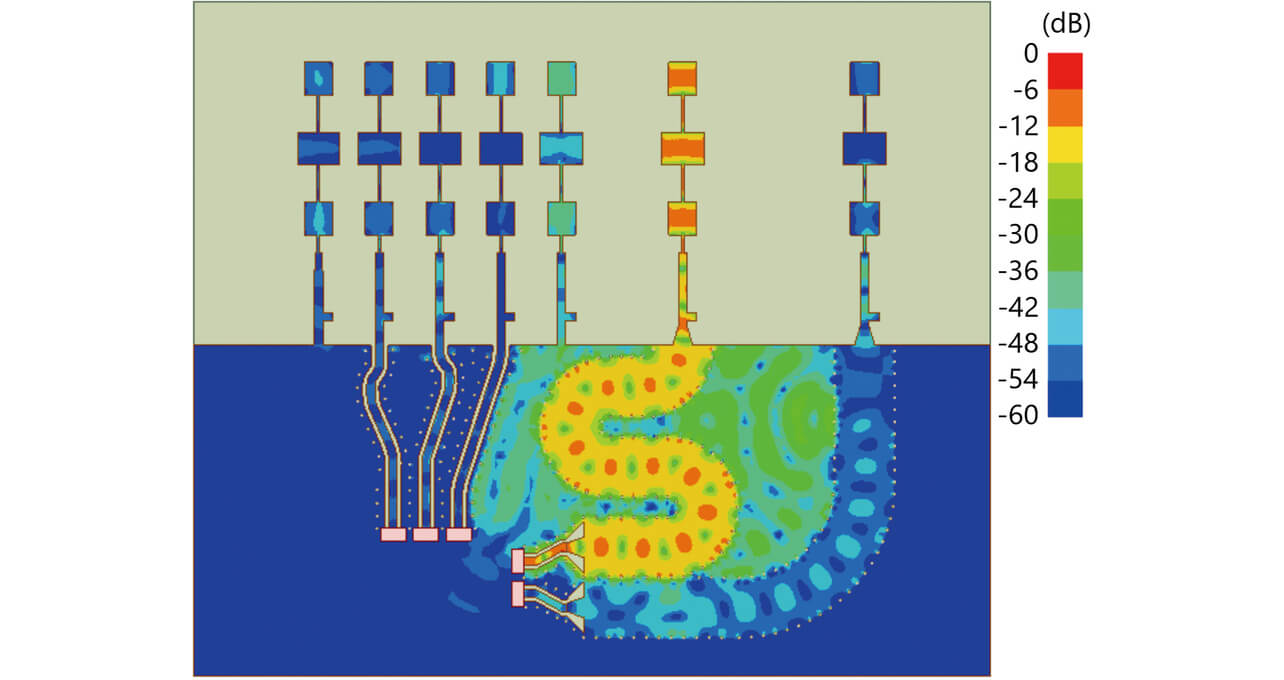
Subsection 4.3 showed that the DOA estimation accuracy improved for most of the azimuth range when the GCPWs were replaced with SIWs. However, the SIW model fared worse for some azimuths, including those near –45° than the GCPW model. The likely responsible factor was unwanted current flows through the parasitic elements due to their proximity to the SIWs. The current distribution simulation results for supplying power supply to the port connected to Tx1 of the SIW model (Fig. 8) also support the estimation that unwanted currents flowed through the parasitic elements.
Then, with the parasitic elements removed, as in Fig. 9, the SIW model improved in DOA estimation accuracy and consequently showed smaller DOA estimation errors for all azimuths than the GCPW model (Fig. 10). In this case, the largest value of DOA estimation error was 1.2°.
The above observations demonstrate that the DOA estimation accuracy improved due to removing the parasitic elements from the antennas in the configuration discussed herein. This finding suggests that DOA estimation accuracy may improve for antennas of other configurations without parasitic elements or with reduced current flows from transmission lines to parasitic elements.
5. Conclusions
In millimeter-wave radar antennas formed on printed circuit boards, high radio-wave radiation from the transmission lines deteriorates DOA estimation accuracy. Hence, we performed an electromagnetic field simulation to quantitatively demonstrate the effects of DOA estimation accuracy improvements that can be made by replacing GCPW transmission lines emissive of high radiation to space with less radiation-emissive SIW transmission lines. More specifically, the DOA estimation error improved from 4.1° for the conventional GCPW model to 1.2° after replacement with an SIW model.
When SIWs are introduced in millimeter-wave radar-based sensing, the position estimation accuracy improves, making it possible to provide millimeter-wave sensing services for detecting targets with higher accuracy in a wide range of fields, including vehicle-borne equipment, transport infrastructure, FA, and healthcare. Moving forward, we intend to verify the effectiveness of SIWs, using actual SIW radars in scenes of use in possible applications.
References
- 1)
- Foundation for MultiMedia Communications, “Overseas Trends in Millimeter Wave Radar (Sensor) Systems and the Like,” (in Japanese), Land Radio Communication Committee, Information and Communication Technology Subcommittee, Information and Communications Council, May 29, 2019, https://www.soumu.go.jp/main_content/000624368.pdf (accessed Feb. 8, 2023).
- 2)
- Information and Communications Council, “Partial Report on the ‘Technical Conditions Relevant to the Diversification of Radio Equipment Using 60 GHz Band Frequency Radio Waves’ among the ‘Technical Conditions Required to Upgrade Low-Power Radio Systems’” (in Japanese), Information and Communications Council, Mar. 30, 2021, https://www.soumu.go.jp/main_content/000741191.pdf (accessed Feb. 8, 2023).
- 3)
- S. Ohashi, Y. Tanimoto, and K. Saito, “3D Imaging of Outdoor Human with Millimeter Wave Radar using Extended Array Processing,” (in Japanese), OMRON TECHNICS, vol. 54, no. 1, pp. 92-100, 2022.
- 4)
- J. Xu, W. Hong, H. Zhang, and Y. Yu, “Design and Measurement of Array Antennas for 77 GHz Automotive Radar Application,” in 2017 10th UK-Europe-China Workshop on Millimetre Waves and Terahertz Technologies (UCMMT), 2017, pp. 1-4.
- 5)
- Y. Fan, M. He, and Z. An, “An Array Antenna for 24 GHz Automotive Radar Application,” in 2020 Int. Conf. Microw. Millimeter Wave Technol. (ICMMT), 2020, pp. 1-3.
- 6)
- Y.-J. Ye, H.-Y. Chueh, W.-C. Chang, and W.-J. Liao, “A Series-Fed Patch Antenna Array for Biomedical Radar Applications,” in 2021 Int. Symp. Antennas Propag. (ISAP), 2021, pp. 1-2.
- 7)
- D. Deslandes and K. Wu, “Integrated Microstrip and Rectangular Waveguide in Planar Form,” IEEE Microw. Wireless Compon. Lett., vol. 11, no. 2, pp. 68-70, 2001.
- 8)
- R. Kazemi, A. E. Fathy, S. Yang, and R. A. Sadeghzadeh, “Development of an Ultra Wide Band GCPW to SIW Transition,” in 2012 IEEE Radio Wireless Symp., 2012, pp. 171-174.
Ansys HFSS is the registered trademark or trademark of ANSYS, Inc., USA or its subsidiaries in the United States and other countries.
The names of products in the text may be trademarks of each company.