


Transfer Learning Technique for Identifying Optimal Production Conditions with Accuracy and Efficiency
- Transfer learning
- Design of experiments
- Support vector regression
- Quality control
- Optimal production conditions
In the manufacturing industry, it is important to identify the optimal production conditions using statistical methods, such as design of experiments. However, the number of experiments is often reduced through the use of knowledge and other means, which leads to lack of accuracy in the response surface model (RSM) for predicting product quality. In this paper, we adopt transfer learning, which is a technique of efficient learning by utilizing the knowledge gained in other domains, to propose a method for constructing RSMs with higher accuracy by introducing past experimental data into the learning process, even when only a few experimental data are available. In addition, we conducted an experiment on a packaging machine to verify its effectiveness. As a result, compared with the RSM constructed on a sufficient number of experiments, the proposed method managed to improve prediction accuracy by about 25%, even when the number of experiments was limited to 1/3.
1. Introduction
High levels of quality assurance and improvement of productivity are required in the manufacturing industry, although workforce shortages are becoming serious. In order to respond to such needs, quality control utilizing the accumulated data from upstream to downstream of the manufacturing process is becoming popular. In the planning and designing phase of the manufacturing process, construction of the manufacturing line that can stably produce quality products is the aim by incorporating the relationships between the manufacturing condition and quality of the product found by the number of experiments in various conditions into the design and manufacturing process. However, a change in the manufacturing environment, such as supplier change, transfer of the manufacturing facility, and replacement of the manufacturing equipment, which are difficult to assume during the design phase, can possibly occur. In recent years, the effect on quality of the product due to the use of the aged manufacturing equipment is also a concern that is caused by postponement of investments in new equipment due to intensified U.S.-China trade conflicts and/or COVID-191). In such a case where the effect on quality can possibly occur, experiments may be conducted to consider changes in the manufacturing conditions and the design.
One of the objects of such experiments is to construct a model representing the relationship between the manufacturing condition and quality. The design of experiments is a common method of such experiments and analyses to construct a precise model efficiently for such purposes. When the design of experiments is conducted, the number of experiments is frequently reduced compared with the recommended number of experiments, which is usually too large, utilizing knowledge2). For that reason, additional experiments become frequently necessary because of inadequate precision of the model due to the effect of factors that are not considered, inappropriate range of the experiments3). Accordingly, to construct a high precision model by number of experiments that is small enough is required in manufacturing industries.
Several methods to construct a high precision model even with a small number of experiments are proposed, and such methods can be classified as the method using knowledge or simulation4) and the method using the data obtained by similar manufacturing process5). Because knowledge is not formulated in many cases in the manufacturing floor, the former method is difficult to use. On the other hand, it is considered that the relationship between the manufacturing condition and the quality will be represented by similar expressions even in the event manufacturing equipment deteriorates, the manufacturing line is transferred as far as the product remains unchanged. Based on such concepts, we have studied the method to construct a model incorporating the data obtained when the manufacturing line of the same product was first started in the past to the data obtained when the event affecting the quality occurs. In this paper, the simple method as much as possible is proposed that is compatible with the complexity of the model encountered in the manufacturing industry.
2. Proposed Method
2.1 Outline of the Proposed Method
The phase from the design of the new product to the completion of the start-up of its manufacturing line is defined as the Start-up Period, and the phase when adjustment of the quality becomes necessary due to the event affecting the quality caused by deterioration of the manufacturing equipment or transfer of the manufacturing facility is defined as the Quality Adjustment Period. The outline of data acquisition and model construction in the proposed method in the respective periods are shown in Fig. 1.
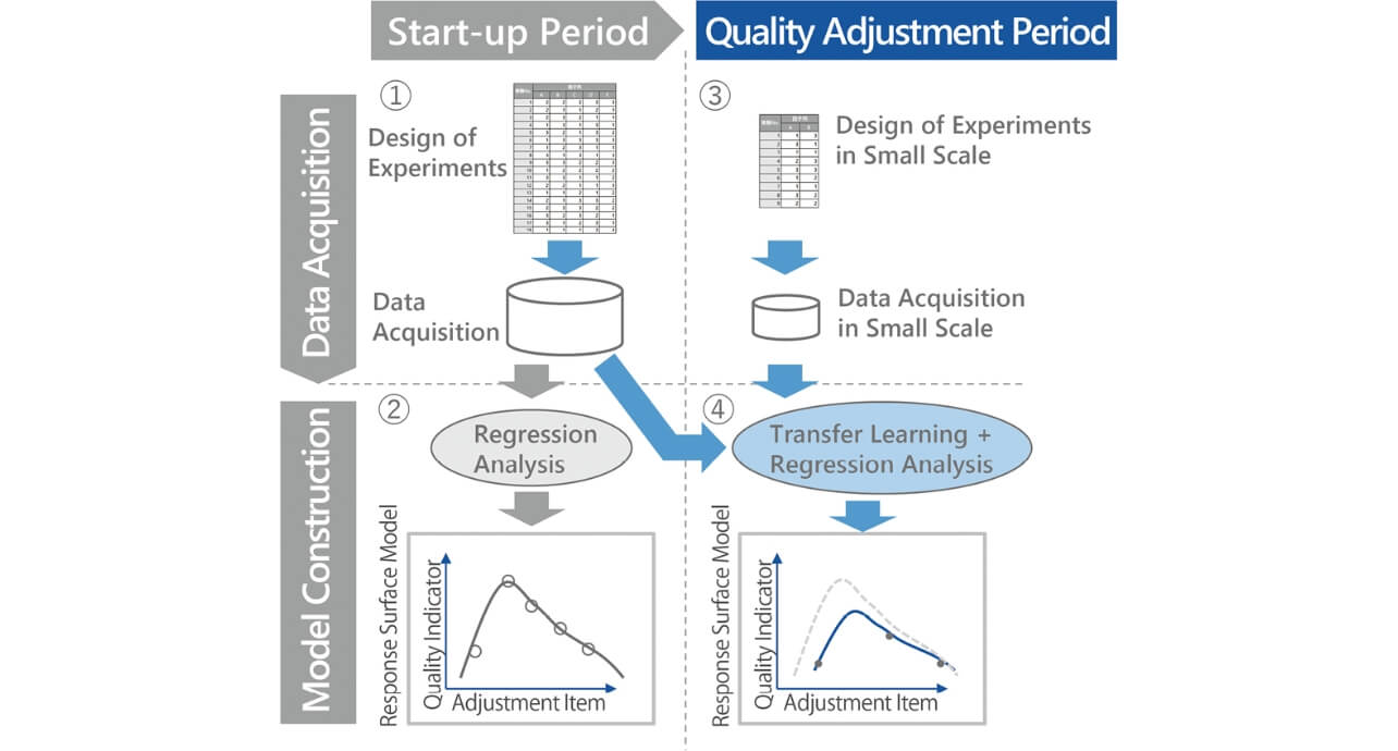
Start-up period:
- (1) Adequate data for all adjustment items are collected according to the design of experiments.
- (2) The Response Surface Model (RSM) is constructed based on the data collected in (1) above, and the optimum manufacturing condition is identified.
Quality adjustment period:
- (3) Data with the number of experiments restricted are collected based on the design of experiments utilizing the knowledge.
- (4) The RSM is constructed by transfer learning based on the data collected in (3) using the data collected in (1) above to adjust manufacturing conditions to the optimum conditions.
The RSM is the model representing the relationship between the manufacturing condition and the quality of the product. The RSM is expressed by Equation (1) involving a function where  is the explanatory variable representing the adjustment item determining the manufacturing condition and
  is the response variable representing the quality indicator determining the quality quantitatively.

ε is the noise. Besides the RSM used for optimization of the manufacturing condition in quality adjustment, the RSM is also used in various applications, such as reduction of tact time for a change in the manufacturing conditions corresponding to the production speed and the pursuit of the manufacturing mechanism.
The objective of this proposed method is to construct the RSM taking the peculiarity of the acquired data in the start-up period into consideration and combining the transfer learning and regression analysis while ensuring the quality of the data acquired by the design of experiments. Construction of the high precision RSM is intended using this method even when only the small scale data are acquired.
From the following subsection, the outline of the concept and application method are discussed for the underlying techniques (design of experiments, transfer learning, and regression analysis) of the proposed method.
2.2 Design of Experiments
The design of experiments collectively means the statistical approach for the method of experiments and analyses of the experiment data to know how the factors (adjustment items) will affect the characteristics (quality indicators) precisely and effectively. The design of the experiments for the combinations of all factors and all levels is called the factorial design, and the design with a reduced number of experiments for the factorial design based on the statistical approach, such as from orthogonality when the number of factors is too large, is called the fractional factorial design. There are a variety of designs for experimental methods depending on the purpose, such as the central composite design considering a balance between reduced number of experiments and quality of the data required to construct the RSM and the optimal design that provides the optimum design under restriction of number of experiments.
In any of the methods, there is a tradeoff between the number of experiments and the expected accuracy of the RSM obtained from the experimental data. When the number of experiments is small, the expected accuracy tends to decrease because the higher dimensional effects and interactions between factors are not considered.
2.3 Transfer Learning
Transfer learning is a method to improve the efficiency of learning in the target domain and to realize construction of the model with a higher accuracy of prediction by incorporating the data and features obtained from the other domain (source domain) when learning is based on the data obtained in the target domain considered.
For transfer learning, hypotheses are made from the aspects of the target domain that are similar to the source domain. When there is little similarity or the transfer learning method is not appropriate from the aspect of similarity, the effectiveness of the transfer learning will not be good because information of the source domain is not transferred properly. In such a case, the effectiveness of the transfer will not be good, and the performance of the transfer will deteriorate, and such a situation is called a negative transfer6).
In this paper, the state of the manufacturing line in the start-up period and the quality adjustment period are treated as the source domain and the target domain, respectively. As it is considered that the RSM in the quality adjustment period has changed from the state in the start-up period, the precise RSM cannot be constructed in many cases by simply combining the data obtained in the start-up period and the quality adjustment period. But the RSM in the start-up period and the quality adjustment period will be expressed by a similar expression because the product manufactured and the manufacturing method remain the same, which is assumed to be a similarity in transfer learning, and the effectiveness of the transfer is expected.
Based on the assumption of such a similarity and the condition setting explained in Subsection 2.1, the following requirements are considered for the transfer learning method.
- To be applicable to the regression analysis
- Number of training data should be from a few tens to a few hundreds (because the number of training data = number of experimental conditions×number of samples, and the number of experimental conditions employed in the design of experiments is usually less than 30).
Many studies of transfer learning are the classification problem (such as image identification) and most of the studies where transfer learning is applied to the regression analysis are related with the deep learning as a prerequisite.
The methods satisfying the above requirements are CORAL (Correlation Alignment)7) and FEDA (Frustratingly Easy Domain Adaptation)8). CORAL cannot handle the nonlinearity of the training data because the method employed is to convert the variance-covariance matrix in the source domain to fit in the target domain. Accordingly, FEDA is used in this paper. FEDA is a method to connect a zero vector to the data of the source domain and the target domain and expand the data three times in the column direction and to handle them as the training data of any learning algorithm as shown in Fig. 2.
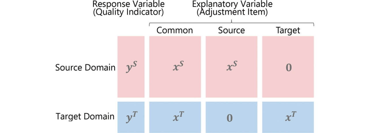
So, no restriction applies in the modeling method. By expanding the data, learning of the features common to the target domain and the source domain and the features unique to either of the target domain or the source domain can be possible while classifying them naturally. As the features taken from the source domain can be controlled like this, it is expected that negative transfer is not likely to occur.
The specific details of processing are as follows. Training data of the source domain and the target domain are expressed by Equation (2) respectively.

Where  ,
,  and
and  ,
,  are the response variables and explanatory variables of the source and target domains respectively, and NS, NT are the number of training data (NS + NT=N ) of the same domains. The training data of the source domain (, ) are expanded to (, 〈, ,0〉) and the training data of the target domain (, ) are expanded to (, 〈, 0, 〉). Learning is made by the usual method after combining the data expanded in the row direction.
It is further possible to expand the data with respect to the feature value φ() by mapping to the higher dimensional space when compatible with the modeling method using the kernel method explained in Subsection 2.4. The feature values φ(), φ() of the explanatory variables , in the source domain and the target domain are expanded to 〈φ(), φ(), 0〉, and 〈φ(), 0, φ()〉respectively. Let ,  as the data in the source domain or the target domain. The kernel function
  (, ) for the feature values expanded can be expressed as Equation (3) using the original kernel function
  (, ) = (φ(), φ()), when calculated for the cases where the domains of the and are the same or different.

Equation (3) means that the weight of the learning from the target domain is calculated as twice as large as the weight of learning from the source domain when the unknown data in the target domain are predicted using the constructed RSM. Accordingly, it becomes possible to predict the target domain with taking the information from the source domain into consideration8).
In this paper the method of learning by usual method in the former case after the data are expanded is called Simple-FEDA (s-FEDA), and in the latter case, the method compatible with the kernel method is called Kernelized-FEDA (k-FEDA).
2.4 Regression Analysis
No restriction applies in the method of regression analysis to construct the RSM, but in the design of experiments, quadratic polynomial regression is usually used. When quadratic polynomial regression is used, the interpretation of the analysis will be easy because the model structure is simple, but the accuracy of the analysis may not be satisfactory if the relationship between the factors and the response is complicated. Accordingly, nonlinear regression is effective if the complicated relationship between the factors and the response is anticipated.
The Neural Network (NN) Regression9), Gaussian Process Regression (GPR)10), and Support Vector Regression (SVR)11) are the major nonlinear regression methods. The NN involves a large number of hyperparameters, which makes learning difficult and takes a long time. In the case of GPR, while the parameter adjustment is easy, a large amount of computation is required, and a complicated model will result because the model is constructed using all the data. In the case of SVR, the parameter adjustment is easy, and a simple model will be obtained because the model is constructed using only some key data. Accordingly, SVR is used in this paper as the regression analysis method.
The SVR is a nonlinear regression analysis method using the kernel method. By the kernel method, learning of the nonlinear relation becomes possible because the data are learned after they are mapped in the higher dimensional space instead of learning them directly. In addition, the following are the points to combine the kernel method with FEDA as explained earlier.
- Model construction by k-FEDA is possible because the kernel method is used (Equation (3)).
- If FEDA and the quadratic polynomial regression are combined, it is equivalent to the modeling for the source domain and the target domain individually, and no effect of transfer can be obtained.
The model expression in SVR is expressed as follows using mapping to the higher dimensional space.

By solving the optimization problem (Equations (5) and (6)) introducing ε-insensitive error by the method of Lagrange multiplier, the model expression (Equation (7)) can be obtained.


Where  and
and  are Lagrange constants and C and ε are hyperparameters. C adjusts the balance between the prediction error and regularization and ε controls the width of insensitive error band. Only the training data effective in expressing the model are extracted owing to the effect of regularization and insensitive errors. Prediction for data is made by the linear combination of values of the kernel function corresponding to some of the training data
  .
.
The Gaussian kernel (radial basis function, RBF), polynomial kernel, and sigmoid kernel are used as the kernel function (, ). There are hyperparameters that determines form of the kernel function and those that will bring the highest prediction accuracy after cross-validation will be generally adopted by the grid search.
3. Preliminary Experiment
The preliminary experiments are conducted for the artificial training data to verify the principle.
3.1 Outline of the Experiments
Details of the training data artificially created are shown in Table 1. Two true models F () are created corresponding to the source domain and the target domain assuming the actual use case. Output  corresponding to the inputs
  (i=1, 2,... Ntrain ) for the source domain and the target domain, respectively, are generated by Equation (8).

Where εi ~ N (0,1) are noise. Number of training data Ntrain is determined so that the ratio between the source domain and the target domain becomes 10:1 assuming that the number of the data is small in the target domain.
| Domain | F (x ) | Ntrain −5≤x≤5 |
Ntest −10≤x≤10 |
|---|---|---|---|
| Source | 0.2x2−0.2x+3 | 100 | |
| Target | 0.2x2−0.3x+0.5 | 10 | 100 |
FEDA (s-FEDA, k-FEDA) is used as the transfer learning method, and SVR is used as the regression analysis method in the configuration of the proposed method to be applied. RBF that allows use of the speeding technique is adopted as the kernel function of SVR, which is explained later. RBF is expressed by Equation (9).

The value y is the hyperparameter that determines the form of the function. Speeding technique proposed in the preceding research is used for adjustment of the hyperparameters C , ε , and γ of SVR12).
The RSM is constructed applying methods (SVR, SVR+s-FEDA, SVR+k-FEDA) whether or not they involve the transfer learning to the training data generated.
3.2 Results of Experiments
The performance of the respective methods is compared predicting the true value of the target domain using the RSMs constructed by such methods. The error is evaluated predicting the true value F () (i=1, ..., Ntest ) for the range of wider than the training data to know the generalization performance. The prediction error is evaluated using RMSE (Root Mean Square Error)(Equation (10)). Where  (i = 1, ..., Ntest ) is the predicted value.

Fig. 3 shows the RSMs constructed, and Fig. 4 shows RMSE by the respective methods as the evaluation results. The shaded area in Fig. 3 is the range of the training data, and the data points are the training data in the target domain.
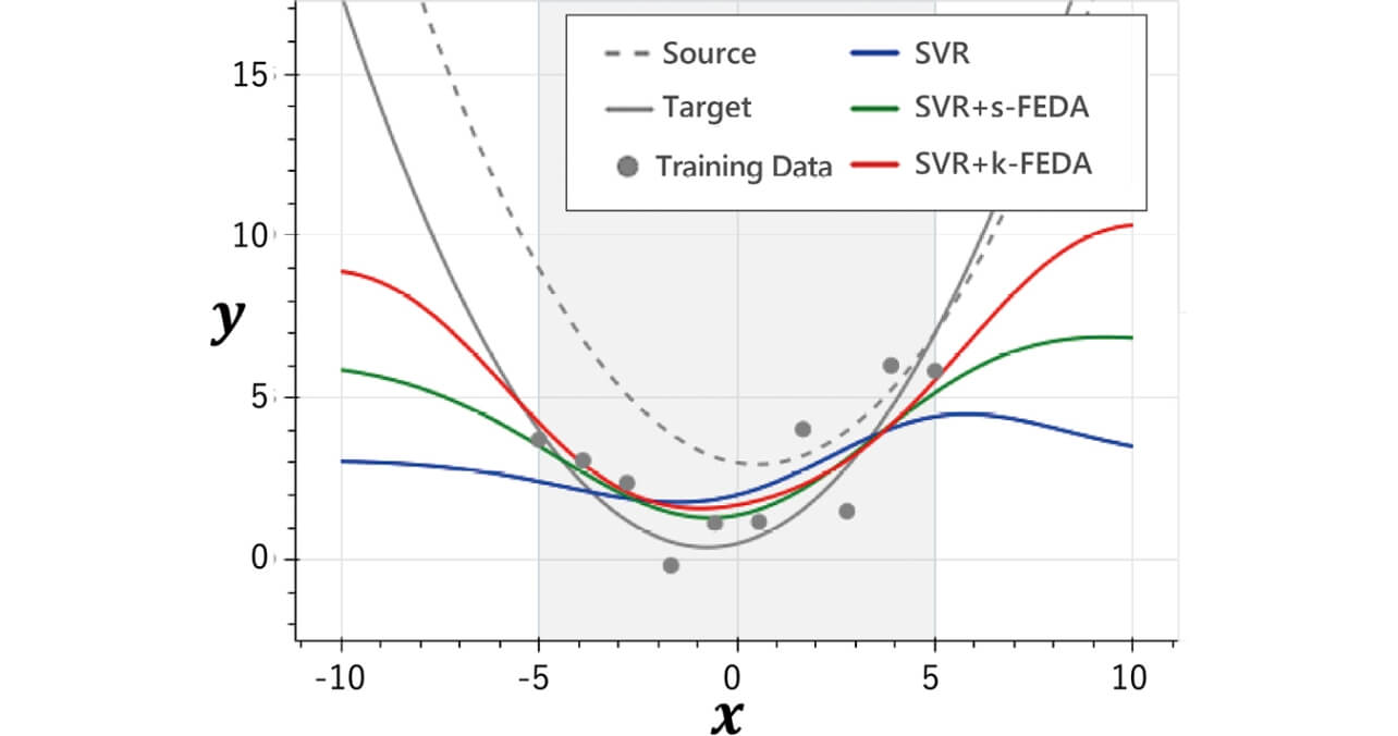
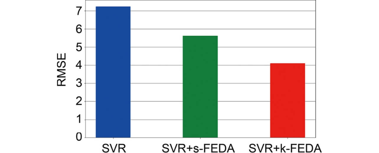
The prediction error is large when the proposed method is not used because the number of training data is small, but when the proposed method (SVR + s-FEDA, SVR + k-FEDA) is used, the prediction error is improved as the training data become close to the model form of the source domain where abundant training data are available. It is confirmed that generalization performance of SVR + k-FEDA is good because the difference from the model form of the source domain is small. It can be considered that different domains result in complicated expressions as mapping to the higher dimensional space is applied after expansion of the data in SVR + s-FEDA while different domains are expressed by simple coefficients in SVR + k-FEDA as shown in Equation (3). As explained above, the RSM of the target domain taking the form of the RSM of the source domain into consideration is expected to be obtained by applying SVR + k-FEDA. Accordingly, SVR + k-FEDA is used in verification of the effect using the actual equipment in the next Section.
4. Verification of the Effect by the Actual Equipment
Verification results of the effect when the proposed method verified in Section 3 is applied to the horizontal form fill seal machine in the experiment are discussed in this section.
4.1 Outline of Verification
Fig. 5 shows the configuration of the horizontal form fill seal machine to which verification of the effect is made.
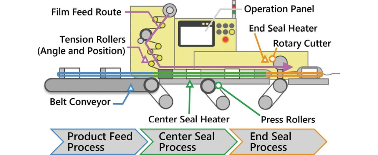
A product enters the packaging machine and is transferred by the press rollers while wrapped by the film formed in a tube shape by the center seal heater. The product is packaged by the film in pillow style after the film located forward and aft of the product is welded in the end seal process and is cut by the rotary cutter. Production of the product is made possible by strictly controlling the temperature and speed using the PLC and by adjusting the machine mechanically according to the machine condition and specification of the product13).
The effectiveness of the RSM constructed by the design of the experiments is verified in this paper, considering the use case where the packaging machine resumes operation after the optimum manufacturing condition is identified when the quality problem occurs due to deterioration of the equipment.
Wear of the press rollers is considered specifically as deterioration of the equipment, where improper welding of the center seal occurs due to wear of the press rollers, which are the components to pinch and feed the film in between. Deterioration of the equipment is simulated by increasing the width of the gap between the press rollers and loosening the adjusting screws because it is difficult to use actually worn rollers.
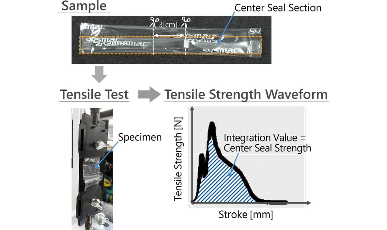
The strength of the center seal is used as the quality indicator corresponding to the quality problem due to wear of the press rollers. Fig. 6 shows the method used to measure the strength of the center seal. The tensile strength of the center seal used as the indicator is measured as the strength of the weld (tensile energy) using the apparatus and the method specified in JIS Z 023814). The specimen taken from the sample is subjected to a tensile test, and the waveform of the strength N is recorded starting from the time the tensile force is applied to the time when the weld is completely destroyed (one stroke), which is taken into the PC as the time series waveform. Then the integration value of the time series waveform for one stroke is calculated as the center seal strength as the quality indicator.
Five adjustment items, packaging speed [CPM], center seal temperature [°C], end seal temperature [°C], tension roller angle [°], and tension roller position [cm] that are adjustable and will affect the quality indicator, are selected. Packaging speed, center seal temperature, and end seal temperature are adjusted from the operation panel. Tension roller angle and tension roller position are the items adjusted mechanically to determine the entry angle and position of the film when the product enters the center seal process.
4.2 Acquisition of the Data for Verification
The data are acquired in three domains (states) during transfer learning—in the start-up period and in the machine deterioration period (small scale) that are the source domain and the target domain, respectively, and the machine deterioration period (large scale) that is used as the reference in verification of the effectiveness.
The start-up period is the state when the packaging machine is started without deterioration and is the case when experiments are carried out for all five adjustment items above. The deterioration period (large scale) is the case when experiments are carried out for all five adjustment items in a condition with the deteriorated machine without restricting number of experiments. The deterioration period (small scale) is the case with the deteriorated machine when experiments are carried out for two adjustment items, packaging speed and center seal temperature respectively, that significantly affect the center seal strength based on knowledge. The composition of the training data of respective domains is shown in Table 2, and the outline of the design of experiments is shown in Table 3. The central composite design is used as the design of experiments method that ensures relatively high modeling accuracy by a smaller number of experiments.
| Item | Domain | |||
|---|---|---|---|---|
| Start-up Period | Deterioration Period (Large scale) |
Deterioration Period (Small scale) |
||
| Training Data | Number of Adjustment Items | 5 | 5 | 2 |
| Number of Experiment Conditions | 31 | 28 | 10 | |
| Number of Data | 358 | 273 | 112 | |
| Test Data | Number of Adjustment Items | 2 | ||
| Number of Experiment Conditions | 5 | |||
| Number of Data | 60 | |||
| Adjustment Item | Domain | ||
|---|---|---|---|
| Start-up Period | Deterioration Period (Large scale) | Deterioration Period (Small scale) | |
| Packaging Speed [CPM] | 12~108 | 5~80 | 12~68 |
| Center Seal Temperature [°C] | 135~200 | 140~200 | 152~200 |
| End Seal Temperature [°C] | 130~200 | 130~200 | 130 |
| Tension Roller Angle [°] | 150~158 | 150~158 | 154 |
| Tension Roller Position [cm] | 9.8~14.6 | 9.8~14.6 | 12.2 |
The levels of adjustment item are established so that many quality products can be included in the adjustment range based on the knowledge specific to the packaging machine, the prior trial results, the range that can be established according to the construction, and the specifications of the machine. Level 3 to Level 5 are actually used for respective adjustment items. For the deterioration period (small scale), constant values of three adjustment items (end seal temperature, tension roller angle, and tension roller position) that are not included in the experiments are used as the values in the standard condition where the quality products were produced in the past (130 [°C], 154°, and 12.2 cm respectively). The level of the end seal temperature in the start-up period and the deterioration period (large scale) is established within the adjustable range with the standard condition (130 [°C]) as the lower limit. This is because that quality welding does not occur, and unpackaged products will be produced frequently when the end seal temperature falls below 130 [°C].
Center seal strength is measured for 12 random samples produced from more than 100 samples operating the packaging machine without feeding the product under the respective experimental conditions. The number of training data is not equal to multiples of 12 because the center seal section is not welded for certain experimental conditions, which results in insufficient number of training data.
4.3 Verification Results
It is assumed that the true model is similar in the start-up period and in the deterioration period because the production method and principle remain unchanged in both cases. The performance of the models is compared under such assumption, constructing the RSM applying the methods to the training data as explained in the preceding subsection, and calculating RMSE as the predicted error for the test data.
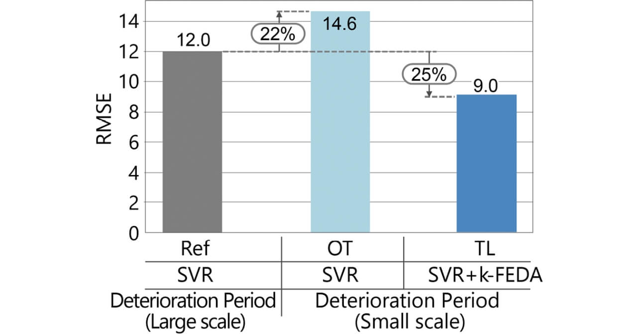
Three RSMs, the model with SVR applied in the deterioration period (large scale) used as the reference (Ref, reference), the model with SVR applied to in the deterioration period (small scale) only (OT, only target), and the model constructed with the proposed method applied in the start-up period and deterioration period (small scale)(TL, transfer learning), are constructed. Table 2 shows the test data used in performance evaluation. The same test data are used for the respective models. Test data are acquired in a manner similar to the manner when the training data are acquired but the experimental conditions of them are different. Constant values in the standard condition of the adjustment items are used for other than the packaging speed and center seal temperature because they do not affect the quality indicator.
Fig. 7 shows the RMSE for the test data of the respective models. The accuracy of OT where the number of the experiments is restricted is 22% lower compared with Ref. However, the accuracy of TL to which the proposed method is applied for the deterioration period (small scale) is improved by 25% compared with Ref.
The time required to construct the model is about 1.5 seconds for Ref. and OT, and about 20 seconds for TL. This will be due to re-computation of the kernel function in Equation (3) because number of training data for TL is larger than the number for other models.
4.4 Discussion
The levels for the training data are established for the start-up period most densely as the number of experimental conditions is larger compared with the other domains. The similarity of the true models in the deterioration period and start-up period is assumed. It is believed that accuracy is improved because the intermediate state between the levels that cannot be expressed by experimental data in the deterioration period (small scale) and the deterioration period (large scale) can be expressed by transfer learning. To enjoy the effectiveness of the proposed method, it is considered important that training data of the source domain are comprehensively acquired, and a similarity of the true models between the source domain and the target domain exists.
As shown in Table 2, the number of experimental conditions in the deterioration period (small scale) is about 1/3 of the number in the deterioration period (large scale) (=10/28). This means that prediction of quality is possible even if the number of experiments is reduced to 1/3 in the manufacturing floor. This means, the man-hour required for quality adjustments can be reduced by two days in the manufacturing floor similar to this verification environment.
The quality indicator of the samples produced is confirmed with the manufacturing condition set as the optimum presumed based on TL. It is confirmed that the mean value of the quality indicator in the presumed manufacturing condition (44.4 [N*mm]) is equivalent to the mean value of the quality indicator (31.5-50.6 [N*mm]) in the experimental condition where the quality products could be produced stably. The center seal strength scarcely changes when the temperature exceeds a certain temperature15). Accordingly, the optimum manufacturing condition for the center seal strength in this verification is considered to be spread extensively, and the manufacturing condition presumed is one of the optimum manufacturing conditions.
As explained above, the proposed method will be able to determine the optimum manufacturing condition with high accuracy in quality adjustment by conducting the experiments focusing on the major adjustment items without the experiments in large scale.
4.5 Issues in the Future
It is impossible to completely eliminate the negative transfer discussed in Subsection 2.4, although the proposed method uses the method to reduce the negative transfer. Negative transfer cannot be identified without the trial conducted under the presumed manufacturing condition with the RSM constructed.
It is desirable that the presence of negative transfer can be identified by the user before the trial under the presumed manufacturing condition considering usability in the actual manufacturing floor. To improve usability, it is considered effective to determine the learning method used according to the prior judgement of the statistical similarity between the learning data in the source domain and the target domain16).
5. Conclusions
The analysis method combining SVR and FEDA is proposed in this paper to construct the RSM with high accuracy even when the number of experiments is limited for the case when quality problems occur because of various varying factors on the automated manufacturing line. In addition, verification of the effectiveness is made to the packaging machine used for the experiment, and it is demonstrated that the improved accuracy of the RSM in the quality adjustment can be expected utilizing the data obtained in the start-up period when various manufacturing conditions are tested.
The authors consider advancement of this method in the future to the technique that meets the variety of needs of the manufacturing industry, such as development of the effective method combining with the active learning and evolution to the optimization of multiple responses taking the variance of the quality indicator into consideration.
References
- 1)
- Ministry of Economy, Trade and Industry, White Paper on Manufacturing Industries (Monodzukuri) 2020. https://www.meti.go.jp/report/whitepaper/mono/2020/index.html (accessed Oct. 30, 2020.
- 2)
- The Japanese Society For Quality Control, Chubu Chapter, Industry and Academia Cooperation Research Group, Statistical Quality Control for Development and Design - Concentrating on Practices by Toyota Group Companies, Tokyo: Heibunsha (in Japanese), 2015, 305p.
- 3)
- H. Morita, Basics and Mechanism of Design of Experiments, Tokyo: Shuwa System (in Japanese), 2010, 278p.
- 4)
- K. Muto and M. Onodera, “Response surface methodology using a prior knowledge and its application to pin fin heat sink design,” (in Japanese), Trans. JSME, vol. 85, no. 880, pp. 19-00194, 2019.
- 5)
- A. T. W. Min et al., “Knowledge transfer through machine learning in aircraft design,” IEEE Comput. Intell. Mag., vol. 12, issue 4, pp. 48-60, 2017.
- 6)
- T. Kamishima, “Transfer learning,” (in Japanese), J. Jpn. Soc. Artif. Intell., vol. 25, no. 4, pp. 1-9, 2010.
- 7)
- B. Sun, J. Feng and K. Saenko, “Return of frustratingly easy domain adaptation,” in Proc. 30th AAAI Conf. Artif. Intell., 2016, pp. 2058-2065.
- 8)
- H. Daume, III, “Frustratingly easy domain adaptation,” in 45th Annual Meet. Assoc. Computat. Linguist., 2007, pp. 256-263.
- 9)
- C. M. Bishop, Pattern Recognition and Machine Learning (vol. 1), Tokyo: Springer Japan (in Japanese), 2012, 349p.
- 10)
- D. Mochihashi, S. Oba and M. Sugiyama, Gaussian Process and Machine Learning, Tokyo: Kodansha (in Japanese), 2019.
- 11)
- C. M. Bishop, Pattern Recognition and Machine Learning (vol. 2), Tokyo: Springer Japan (in Japanese), 2012, 433p.
- 12)
- H. Kaneko and K. Funatsu, “Fast optimization of hyperparameters for support vector regression models with highly predictive ability,” Chemom. Intell. Lab. Syst., vol. 142, pp .64-69, 2015.
- 13)
- K. Tsuruta, T. Minemoto and Y. Hirohashi, “Development of AI Technology for Machine. Automation (1),” (in Japanese), OMRON TECHNICS, vol. 50, no. 1, pp. 6-11, 2018.
- 14)
- K. Hishinuma, Basics and Practices of Heat Seal - Measurement Method of Melting Surface Temperature: Use of MTMS, Tokyo: Saiwai Shobo (in Japanese), 2007, 197p.
- 15)
- Japan Packaging Institute, Packaging Technology Handbook, Japan Packaging Institute (in Japanese), 2019.
- 16)
- Mega Chips, K. Nishiyuki and H. Fujiyoshi, “Clustering Device and Machine Learning Device,” (in Japanese), no. 6516531, Oct. 10, 2016.
The names of products in the text may be trademarks of each company.