


Development of Temperature Prediction Technology for Early Detection of Panel Abnormalities
- Machine Maintenance
- Predictive maintenance
- Thermal monitoring
In recent years, power outages and ignition accidents caused by abnormal temperature rises in panel components due to aging of facilities have been increasing. Consequently, for example in a factory, the production line is shut down, which may lead to losing opportunities and decreasing the public image. Although periodic maintenance by maintenance personnel suppresses the frequency of abnormalities, there will be temperature abnormalities that can progress in a few days, so it cannot be completely suppressed. Therefore, the need for remote monitoring of the temperature by constant setting temperature measuring devices, such as thermocouples or infrared sensors, is increasing.
On the other hand, in cases of abnormalities that lead to ignition or smoke in a few hours, maintenance personnel may have no time to handle the abnormalities on-site after abnormal temperatures with a temperature monitoring device are detected. Also, countermeasures may not be implemented within the time required. Therefore, further early detection of abnormalities is needed. The authors have worked on the early detection of temperatures and developed a predictive temperature function that predicts the final temperature by considering temperature changes in an abnormal device. By realizing the early detection of abnormalities, we achieved the creation of sufficient time so that users can implement the appropriate measures before the occurrence of ignition accidents or power outages.
In this paper, we will give an overview of reaching the predictive temperatures and the technical method to achieve it.
1. Introduction
In recent years, maintenance work has been on the increase with the aging of factory equipment1). Besides, the ongoing population decline and associated factors are making it harder for Japanese enterprises to secure additional maintenance personnel. As a result, the maintenance workload per person likely has increased, and undermaintenace is causing problems of equipment power outages and ignition accidents more frequently than before2). If any manufacturing line should stop and take a long time before recovery, the resulting opportunity losses may seriously affect business management. Should an ignition accident occur as a consequence, the reputation of the company would be compromised. As a preventive measure against such a situation, periodic equipment maintenance is performed by maintenance personnel to reduce the frequency of the occurrence of abnormalities. Some types of temperature abnormalities take several days to unfold and hence may sometimes occur between periodic inspections and fail to be nipped in the bud. Accordingly, needs are increasing for remote temperature monitoring by permanently installed temperature measuring devices, such as thermocouples and infrared sensors.
Meanwhile, some other types of temperature abnormalities take only a few hours to result in a serious accident, such as a sudden equipment stoppage or ignition. In some cases, users may fail to arrive in time to deal with an abnormal temperature on-site after its detection by a temperature monitoring device because of too short a lead time to do so. Thus, the issue to be addressed is to provide a method of detecting abnormalities at a much earlier stage.
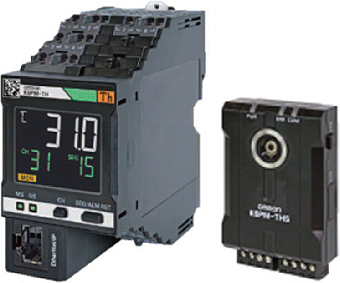
To solve maintenance issues, such as those mentioned above, an early detection technology for abnormalities that unfold in a few hours was established as an achieved-temperature prediction technology. This paper presents this achieved-temperature prediction technology. As a solution to the above issues, an in-panel monitoring device K6PM-TH was developed and implemented with the achieved-temperature prediction technology as one of the main unitʼs functions (Fig. 1).
2. Challenges
2.1 Types of abnormality modes
Interviews with 20 maintenance persons from factories feeling the need to improve maintenance work efficiency found that among in-panel parts and components, those with a particularly high frequency of abnormalities are above-50A high-current relay terminal cables, transformers, and inverters. Hence, these products are the ones to be analyzed for abnormality modes.
These parts and components have more than one abnormality mode. Their abnormality modes fall broadly into two categories, one being the progressive abnormality mode and the other being the sudden abnormality mode. In the progressive abnormality modes, chemical changes (corrosion, migration, etc.) due to environmental factors, such as gas atmosphere and humidity, or mechanical changes (cracks, poor contacts, etc.) due to mechanical stress unfolds with a gradual temperature rise over several days to several decades until the eventual failure as typically seen in insulation deterioration.
Meanwhile, a sudden abnormality mode leads to a failure in a few hours when the panelʼs internal temperature increases because of a heat buildup due to a loosened terminal screw (a mistake made by maintenance personnel) or because of an air-cooling fan failure.
2.2 Conventional detection methods
The maintenance detection methods for ignition accidents or thermally induced failures that may occur inside a panel fall into either the portable method involving temperature measurement performed on-site by the maintenance personnel with a thermoviewer or the permanently installed method involving temperature monitoring performed by a permanently installed temperature measuring device, such as a thermocouple.
2.3 Countermeasures for abnormality modes
Progressive abnormality modes unfold with a gradual temperature change over several days to several decades and hence can be solved by monitoring the temperature trend using a permanently installed detection method. The sudden abnormality modes lead to an equipment stoppage or ignition within a few hours after the onset of an abnormality. Therefore, the lead time for the maintenance personnel to perform a remedial repair of the in-panel equipment and safe shutdown thereof can be secured by predicting the final achieved temperature and detect the abnormality at an early stage before the eventual temperature is reached.
Table 1 sums up the detection methods for the two-mode types. This study aimed at establishing a technological solution that allows early detection of sudden abnormality modes undetectable even by permanently installed type devices. At the same time, checks were made to ensure that the solution would not falsely respond to the other types of abnormality modes.
| Abnormality mode | Example | Unit of progress | Portable type | Permanently installed type |
|---|---|---|---|---|
| Progressive | Corrosion, migration, crack, poor contact (rate of progress variable depending on environment) | Years or months | Detectable | Detectable |
| Days | Undetectable | Detectable | ||
| Sudden | Loosened terminal screw (mistake made by maintenance personnel) Air-cooling fan stoppage | Hours | Undetectable | Undetectable |
The indicators of evaluation for our proposed problem solution are the notification lead time from the onset of an abnormality until its detection by our proposed technology and the notification accuracy for securing the reliability of the content of the notification. These indicators are collectively called notification performance. The next two sections provide the details of these indicators.
2.5 Notification lead time
A temperature rise test revealed that an abnormality in a high-current cable, a transformer, or an inverter takes at least 60 minutes from onset until the equipment surface temperature rises to the temperature that poses a risk of failure. This 60-minute lead time was verified by measuring the time from the switching on or loading of the relevant equipment such as an inverter until temperature saturation.
The time necessary for maintenance personnel to head to the site upon the detection of an abnormality and determine the measure to be implemented, such as stopping or repairing the equipment, may vary depending on the distance to the site. The results of the hearing mentioned above showed that more than 90 percent of factories need 15 minutes for maintenance personnel to arrive at the abnormality occurrence site and an additional time of approximately 15 minutes for them to identify and analyze the cause and implement a measure. It follows then that it takes 30 minutes from the onset of an abnormality until the completion of the remedial measure. Because the temperature that poses a risk of failure is reached in 60 minutes, the function desired here must be able to inform the user of an abnormality within 30 minutes from onset.
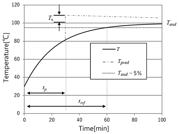
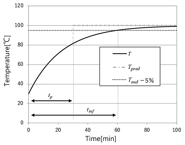
In what follows, the final achieved temperature to be reached after the occurrence of an abnormal event is represented as  [°C], the achieving time for the actual temperature
  to reach ×0.95 (also given as -5%) is represented as
  [min], a predicted achieved temperature (hereafter predicted temperature) is represented as
  [°C], the time required to complete a prediction (notification lead time) is represented as tp [min]. The target to be achieved is
  ≤ 30 minutes. Fig. 2 shows a graphical summary of the parameters for when = 100°C.
2.6 Notification accuracy
As shown in Fig. 2, the error between the actual final achieved temperature and the predicted temperature is defined as the notification accuracy  (=−). Our proposed achieved-temperature prediction function is intended to prevent equipment stoppage from leading to opportunity losses, ignitions, and smoking. Hence, this function is designed with greater importance placed on false-negative detection, which occurs when an abnormal value is erroneously determined as normal, than false-positive detection, which occurs when a normal value is erroneously determined as abnormal. Where a temperature sensor is used for measurement, the notification accuracy also depends on the rated accuracy unique to the sensor. Therefore, with the rated accuracy of the temperature sensor taken into account, the target error margin for the minus side is defined as -5°C to prevent false-negative detection as much as possible.
Plus-side errors cause overnotifications and increase the number of wasted person-hours for maintenance personnel. Among the in-panel resin materials, the material that most easily burns and emits smoke is polyvinyl chloride (PVC) used for cabling and is said to have a thermal decomposition temperature of approximately 180°C. To be on the safe side, the temperature that poses an ignition/smoking risk is defined as 100°C or more. Almost all in-panel devices have a design operating temperature range of 50°C or less. Accordingly, the temperature of 50°C is regarded as the upper limit for the operating environment temperature. Besides, the results of an experiment showed that when products for in-panel use are used at the maximum specified load in an environment at 50°C, their surface temperature remains at 80°C maximum. Therefore, standard products for in-panel use are deemed to have an operating surface temperature range of 80°C or less. Let us here rename the above three temperature ranges as Steps 1 to 3. Then, Step 1 is the operational temperature range below 80°C, Step 2 is the warning range from 80°C to less than 100°C, and Step 3 is the emergency response range of 100°C and more. Note that the warning range is a temperature range in which a measure should be implemented to reduce the temperature of the monitoring target because a greater amount of heat than normal has built up in the monitoring target, while the emergency response range refers to a temperature range in which the monitoring target is already at a failure risk and in the immediate need of a countermeasure. In practice, if no error occurs beyond the range of Step 2, no false-positive detection of a Step 3 class temperature occurs in Step 1. Nor does a transition to emergency response occur. Even if the predicted temperature is in Step 3, and the actually achieved temperature is in Step 2, the result will be a notification that the temperature is in the warning range. This notification may lead to a measure for improvement and, therefore, will not result in a complete waste of person-hours. Accordingly, the target notification accuracy set for the plus side is an error margin of +20°C or less, which is the range of Step 2. Thus, the target to be achieved is -5°C ≤ ≤ 20°C.
2.7 Challenges for handling sudden abnormality modes
The following three were set as the challenges to be solved to achieve the notification performance given as the target:
- (a)
- Developing a thermal model of temperature change due to a sudden abnormality mode
Determining by calculation the parameters unique to the product from the measured temperature data to develop a thermal model that allows prediction of the achieved temperature; - (b)
- Predicting the achieved temperature using the thermal model
Developing a prediction algorithm that meets the target “notification lead time” specified above; - (c)
- Improving the prediction accuracy Developing a prediction algorithm that meets the target “notification accuracy” specified above.
3. Development of the achieved-temperature prediction function
3.1 Thermal modeling
For thermal modeling, a control theory-based temperature prediction model was developed. Among the known methods of control theory-based temperature prediction is a technique of instantaneously predicting human body temperatures by clinical thermometer3). In the case of a clinical thermometer, the heat source (=human body) keeps a constant temperature, thus allowing the adoption of a model in which the structure between the human body and the instrument has a constant heat capacity or thermal resistance (i.e., transfer function). In the case of the panelʼs internal temperature monitoring, however, the monitoring target has a gradually rising temperature and hence an unknown transfer function. Accordingly, unknown parameters must be calculated based on the measured temperature to make a temperature prediction.
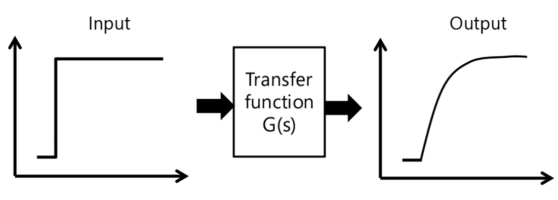
In a sudden abnormality mode, temperature instantaneously changes from a normal to an abnormal state. This change in state is called a stepped change of state. It is a generally known fact that this temperature change is a primary delay system4). This is obvious from Fig. 3 that shows the primary delay waveform for the temperature change measured when a DC power supply generally used in a control panel was driven under constant load.
The transfer function for the primary delay element is given as Equation (1), where  is the Laplacian operator,
  is the gain constant, and is the time constant:

Fig. 4 shows a time response output that occurs in response to a step-shaped signal input. This response is generally called an indicial response or step response. In the case presented here, the input means the onset of an abnormality.
The time response is obtained from Equation (2) below:

The rate of change for the step response  in Equation (2) can be obtained by the time differentiation of Equation (2). The time differential equation is given as Equation (3) below:

This rate of change  is a ratio given in Equation (4) when the time has elapsed by
  from time
  :
:

Hence it follows that the decay rate is constant at any point of time if the elapsed time is constant. This means that the rate of change is times  when has elapsed. When
  is substituted for
  for generalization, Equation (4) is represented as Equation (5). Fig. 5 shows a graphical representation of Equation (5).

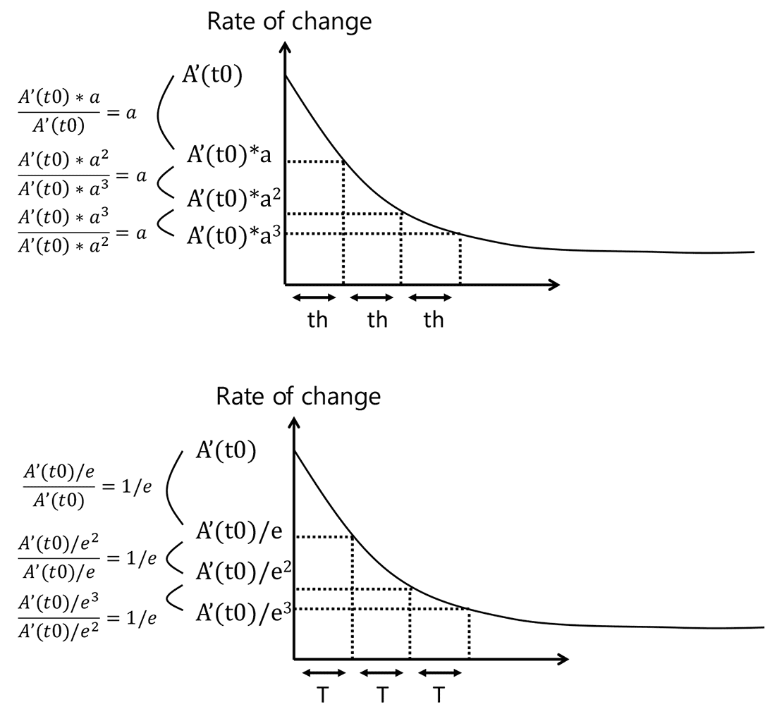
From Equation (5), the temperature change rate after the elapse of time from time  is expressed by Equation (6). This allows prediction of the rate of change at an optional time by finding the time
  for when the temperature change rate has changed by the ratio
  .
.

The amount of temperature change from time can be determined by integrating the temperature change rate with
respect to the time from time until the elapse of . First,  and
and  at a point of time and the decay time of the rate of change are calculated. The decay time is the time required for the change rate ratio to reach . The temperature convergence value (predicted temperature), =
  ( →
( →  ), which has and as the initial values and changes at a constant decay time , can be calculated by Equation (7) below. Note that is represented as t here for convenience.

Thus, the thermal model for calculating the predicted temperature was successfully developed by determining the decay time .
3.2 Prediction algorithm
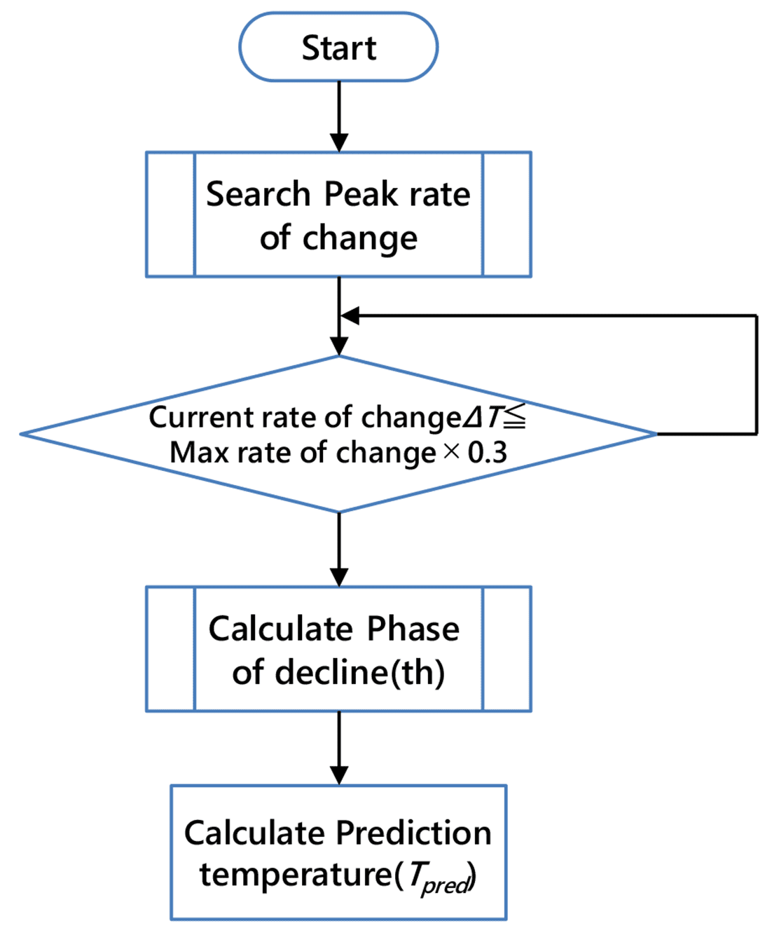
For the verification model case, let the normal temperature be 30°C, the abnormal temperature = 100°C, and the achieving time = 60 minutes. It turned out that the predicted temperature can be calculated by determining th. It is obvious from Fig. 5 and Equation (5) that can be calculated from the elapsed time until the rate of change at a point of time t is times .
As can be seen from Fig. 5, the temperature change rate becomes largest immediately after the onset of an abnormality. Hence, from the maximum temperature change rate, the fastest prediction can be achieved by letting the time until the rate of change is times itself be . Here, = .
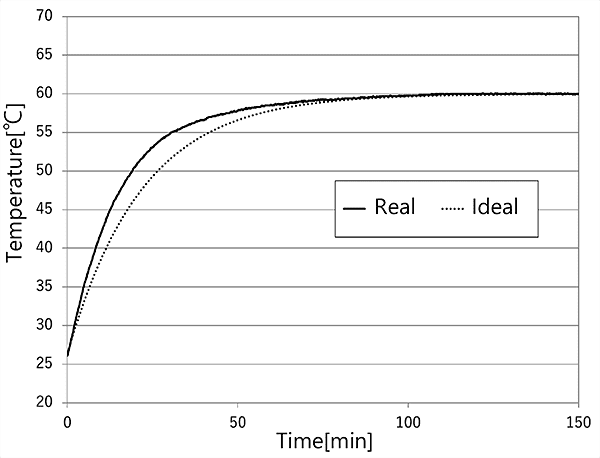
The calculation results obtained by applying the above to the model case so that = ≤ 30 minutes revealed that ≤ 30 minutes or less, if = 0.3. Fig. 6 shows the results of the simulated temperature change. Note that even when > 100°C, the same holds because the temperature change is still a primary delayprocess. Substitution of the results for when = 0.3 into Equation (7) yields Equation (8). Note that log stands
for natural logarithm.

From the above, the predicted temperature can be obtained from Equation (8), using the temperature and temperature change rate at time t0 and the decay time th of the rate of change.
Fig. 7 shows the processing flow for the above.
3.3 Achieved-temperature prediction by the temperature sensor
Table 2 shows the performance of K6PM-THS, a temperature sensor developed at the same time as our proposed solution presented herein.
| Item | Performance |
|---|---|
| Rated accuracy | ±5°C |
| Maximum variation between two consecutive measured values | 1°C/s |
Equation (8) shows that the temperature change rate significantly affects the accuracy of the predicted temperature.The two consecutive measurements taken by K6PM-THS of the maximum rate of change were 1°C/s or less. When =30 minutes, =1°C/s, and the minimum sampling time of 1 second are applied from the primary delay temperature change profile examined in advance, the predicted temperature is given as =+1°C×0.83×30×60=+1494°C from Equation (8). In other words, a fluctuation of 1°C/s in the
measured temperature value means that the predicted temperature changes by 1494°C. To reduce the influence of this fluctuation in the measured temperature value, a digital filter is applied to the measured temperature to perform noise cancellation.
The digital filter is represented by the following Equation (9):

where


where  is the time constant, and
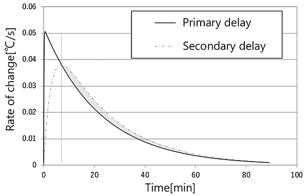
  is the reference sampling time (1 second here). Bear in mind, however, that the reading lags in time more behind the real-time temperature with the increase in this time constant . In other words, an increasing delay occurs to the notification lead time. This problem can be dealt with by adjusting the decay ratio of the rate of change to reduce the value of = by the amount of delay in the notification lead time. Moreover, as shown by Equation (9), our digital filter is a primary delay filter used to damp noise. Hence, a secondary delay may occur through multiplication with the primary delay temperature rise in the product. As is clear from Fig. 8, after the calculation of the maximum rate of change, the secondary delay shows a higher rate of change than the primary delay. This is because the rate of change after filtering lags in time more with the increase in the filter time constant. As a result, the predicted temperature becomes a larger output and negatively affects notification accuracy. This problem can be dealt with by adjusting the time constant to meet the required
notification accuracy.
is the reference sampling time (1 second here). Bear in mind, however, that the reading lags in time more behind the real-time temperature with the increase in this time constant . In other words, an increasing delay occurs to the notification lead time. This problem can be dealt with by adjusting the decay ratio of the rate of change to reduce the value of = by the amount of delay in the notification lead time. Moreover, as shown by Equation (9), our digital filter is a primary delay filter used to damp noise. Hence, a secondary delay may occur through multiplication with the primary delay temperature rise in the product. As is clear from Fig. 8, after the calculation of the maximum rate of change, the secondary delay shows a higher rate of change than the primary delay. This is because the rate of change after filtering lags in time more with the increase in the filter time constant. As a result, the predicted temperature becomes a larger output and negatively affects notification accuracy. This problem can be dealt with by adjusting the time constant to meet the required
notification accuracy.
Under the worst-case conditions, and were determined so that they could meet the required notification lead time. The worst-case conditions occur when two consecutive measured results show a rise at the rate of 1°C/s immediately before the value of the right term on the right side of Prediction Equation (8) becomes largest. Accordingly, the worst-case conditions were applied to the model case to run a simulation. The simulation results show that the required notification performance can be achieved when = 0.5 and = 3 minutes. Table 3 shows the notification performance simulation results thus obtained. As explained with Fig. 8, it is evident that the calculation does not yield the predicted temperature on the minus side with a secondary delay as a factor. The error depends on the rated accuracy of the sensor. The obtained notification accuracy falls within the target accuracy range – 5°C ≤ ≤ 20°C and is acceptable.
| Notification lead time tp [min] | Notification accuracy Ts [°C] |
|---|---|
| 25.1 | +14.1 |
4. Experimental results
4.1 Verification results
Using the infrared sensor K6PM-THS developed this time, field performance evaluation tests were performed on the monitoring targets with various abnormality modes produced. Table 4 shows the monitoring targets and abnormality modes.
Because it is difficult and dangerous to simulate actual ignition/smoking or failure-equivalent abnormalities, the temperature rise range was examined for abnormality modes with a moderate achieved temperature range from approximately 40°C to 60°C compared to the model case. Note also that the power supply and the solid-state relay (SSR) tested for comparison with such devices as the inverter, which is the subject of interest of this paper, are smaller in mass and quick to reach temperature saturation. A primary delay model is a linear model by nature and is known to be analog in the direction of time or temperature when the time constant or the gain constant is multiplied by a constant factor2). In other words, by the nature of the primary delay model, when is multiplied by a constant factor, so is . Therefore, a ratio equal to ≤ 30 minutes for the target numerical value of = 60 minutes was used to achieve a target notification lead time that satisfies the condition ≤ /2. The target notification accuracy range to be achieved was – 5°C ≤ ≤ +20°C.
Table 5 shows the verification results, revealing that the target notification performance was achieved under the conditions of all the cases.
| Monitoring target | Abnormality mode | Details |
|---|---|---|
| Power supply (60 W) | Poor contact due to a loosened terminal screw | Turn ON the power with the screw loosened |
| SSR (rated current: 20 A) | Fan stoppage | Turn ON the power and warm up the fan at 100 percent of the rated current. Stop the fan when the temperature stabilizes. |
| Contactor (rated current: 25 A) | Overload | Turn ON the power at 100 percent of the rated current. |
| Monitoring target | Abnormality mode | Notification lead time | Notification lead time Ts [°C] | |
|---|---|---|---|---|
| Notification accuracytp [min] | Achieving timetinf [min] | |||
| Power supply | Poor contact due to loosened terminal screw | 12.0 | 25.0 | +2.1 |
| SSR | Fan stoppage | 13.5 | 27.5 | +1.1 |
| Contactor | overload | 19.0 | 45.2 | +1.5 |
5. Conclusions
Our proposed unique achieved-temperature prediction technology allows early detection of temperature abnormalities during the sudden abnormality modes. Moreover, this technology meets the required notification performance and hence can provide maintenance personnel with the lead time for them to improve or repair problems in panels before an accident or a fire occurs. Thus, our proposed technology enables early detection of abnormal temperatures in high-current cables, transformers, and inverters said to have a particularly high frequency of abnormalities.
The K6PM Series in-panel monitoring device provides a lineup of compact, wide-view-angle temperature sensors necessary for in-panel monitoring. Besides the achieved-temperature prediction function explained above, the main unit features a function for canceling the influence of outdoor air temperature and a function that automatically sets the temperature threshold for determining the occurrence of abnormalities. We believe that this technology helps to realize man-hour-saving temperature monitoring without reliance on personal skills, minimize the need for reactive maintenance, and allow the transition to preventive maintenance.
In the future, we intend to make shorter decay time settings available to allow further earlier detection of panelsʼ internal temperature abnormalities. For this purpose, we will add enhanced accuracy to our temperature sensors and develop noise cancellation technology.
References
- 1)
- Semiconductor Manufacturing Technology Committee, Japan Semiconductor Committee, JEITA Semiconductor Board, “Overview of Operational Risks of Semiconductor Manufacturing Lines During Long-Term Use of Silicon Wafer Cutting Machines for Silicon Wafers Sized 200 MM or Less” (in Japanese), p. 5, 2012.
- 2)
- Tokio Marine & Nichido Fire Insurance Co., Ltd., “Forefront of Risk Management” (in Japanese), 2012, p. 3.
- 3)
- OMRON Corporation, “Electronic Clinical Thermometer,” Japanese Unexamined Patent Application Publication. No. 60-209125, 1985-10-21.
- 4)
- K. Bunji, Fundamentals of Control Engineering, Morikita Publishing, pp. 35-36, 1977.
The names of products in the text may be trademarks of each company.