


AI Visual Inspection System
- AI
- Deep Learning
- Visual Inspection
- CPU Optimization
In this paper, we propose a technique to detect various defects in uniform background objects (hairline, satin, etc.) in visual inspection system. “Human resources shortage” and “ diversification of consumer needs” have emerged recently in the field of manufacturing, and the demands for the autonomous visual inspection system are increasing. The existing inspection system, however, cannot adapt to a wide variety of objects / defect types. We built Deep Learning model that learns a variety of defect types in advance, thereby constructing a defect detection system that enables anyone to automatically perform inspection like human eye without any complicated setup. In addition, without introducing high-cost computing resources such as GPU, it can be feasible on existing vision system by highly optimizing for modern CPU.
1. Introduction
1.1 Background
In the field of manufacturing, human resource shortages and diversification of customer needs have become more diversified, and demand for automatization of visual inspection systems has been increasing. Existing image sensors, however, have only made part of the automatization of inspection processes feasible. The causes include the following: such sensors cannot adapt to diverse materials and shapes for the objects to be inspected owing to a wide variety of objects to be manufactured; and adjustment is not possible unless sophisticated expert knowledge is available. To this end, our goal is to achieve automated visual inspection technology that satisfies the requirement to be applicable to a wide variety of objects and defect types and can be setup easily by anyone for the automatization of inspection processes.
To deal with a variety of objects and defect types, the algorithm to detect defects, input (lighting/imaging) technologies that highlight defects, and the driving technology to adapt to object profiles are necessary. In this paper, we propose a defect detection algorithm for the detection of diverse defects.
1.2 Proposal for pre-training type defect detection using deep learning
Under the circumstances where the deep learning method brings results in a variety of image analyses, the bottleneck is the collection of images. For practical realization of deep learning for visual inspections, the collection of images used for learning will constitute a great burden for fieldworkers, thereby making it difficult to secure a sufficient number of learning images when starting the product line. In this paper, to resolve the problem, we propose the automatization of visual inspections wherein the pre-training type algorithm that does not require preparation of learning images for each product line is applied.
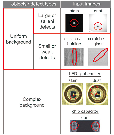
In the visual inspection, it is necessary to detect only defects from a small or weak difference in a variety of object surfaces and defect types. The objects and defect types subject to visual inspection can be classified as shown in Table 1. Out of the classified inspections, the inspection that has been put into practical use with existing image sensors is limited to salient defect inspections under a uniform background. On the other hand, the algorithm proposed in this paper can be applied to small or weak defects in the uniform object. Because a uniform object shows similar features even across different product lines, the pre-training type algorithm can work well.
2. System outline
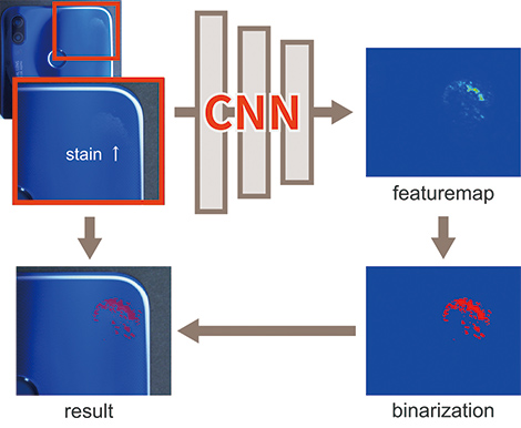
Fig. 1 is an illustration of detection processing. The feature map expresses the likely level of defects by processing the input image with the pre-training type of a convolutional neural network (CNN). Thereafter, the feature map thus obtained is binarized and extracted as a defect region.
Study cases of deep learning for implementing such tasks are often based on algorithms that include object detection and semantic segmentation to output the processing results1). On the other hand, the algorithm proposed in this paper sets out the feature map as the final output. The reason for this is that, for the actual production sites, the judgment regarding whether defects in products are classified as defective products or accepted as good products is different for each product line, and thus it is necessary to leave room for setting the threshold values for the respective lines. The actual operation model assumes that the algorithm is used as part of a series of inspection flows, after generating the feature map wherein only the defective portions are highlighted by the proposed algorithm, and on board the image sensor, binarization or labeling of simple image processing is applied; thus, the acceptance judgment is implemented by using the positions and sizes of any defects.
3. Algorithm for generating defect detection image
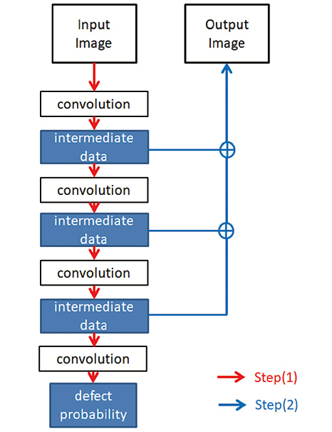
In the defect inspections implemented at manufacturing sites, the assumption is that objects other than defects may be projected in the images, and there may be cases that require classification of defects and other objects in the post-processing stage. Therefore, it should be so arranged that the positions and sizes can be identified by the feature map wherein the likely level of a defect is imaged. Preparation of such a feature map consists of the two steps shown below (Fig. 2).
- (1) Assumption of the probability that a defect is in the inspection image
- (2) Identification and imaging of the estimated position of the defect
First, for step (1), enter the inspection image into CNN and output the possibility that a defect can exist within the image with a probability of 0 to 1. CNN is so arranged that it outputs high values when patterns that are closer to defects are contained in the inspection image by allowing advance learning from many defect images.
Next, for step (2), it is determined from which place within the inspection image the probability of the defect estimated in (1) is derived. With CNN, the information showing the positions of defects are contained in the calculation results of the respective intermediate layers2), and by using the information, the degree of contribution to defect probability can be calculated in units of inspection image pixels. Finally, the degree of contribution from each pixel is multiplied by the adequate magnification ratio, thereby creating the feature map.
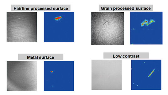
Fig. 3 is an example of a feature map. In this illustration, the color varies from blue to red as the degree of contribution to defect probability becomes higher. It is known in the inspection image that the portions where defects exist show higher values.
4. Learning image database
To allow the pre-learning type algorithm to exert full performance, it is necessary at the time of development to build a large database (DB) of learning images that covers a variety of objects produced at the manufacturing site. However, since the actual product line data are not always saved, and such data may often be confidential, data collection for the purpose of development use is not easy. In particular, for image data that contain defects, there are also problems where the absolute number is small and the volume of data for good products is not balanced.
As a method for building the DB under the condition where images usable for learning can be procured, a method of pseudo images generated by computer graphics (CG) or generative adversarial network (GAN) are used as the learning images3),4), but cases where validity is practically shown in the actual environment are rare.
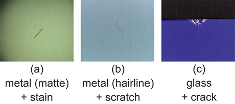
Therefore, referring to the development of the algorithm proposed in this paper, patterns of objects where combinations of defect types, positions, sizes, colors, background materials, and light source setups are included were actually created and imaged, thereby building the DB. Fig. 4 shows examples of combination patterns actually created.
For the processing of learning, images obtained by adding data augmentations that included clipping and the addition of noise to each image recorded were used after increasing the number of images to 8 million. The use of the DB allows the algorithm proposed in this paper to handle a variety of objects and defect types at the manufacturing sites.
5. Considerations on higher speeds
In general, abundant computational resources from the GPU are used to implement deep learning. For image sensors used at the manufacturing sites, however, the use of such resources is difficult because of such problems as cost. Therefore, to improve high-speed performance through processing with a CPU, attention focused on the convocation layer that accounted for CNN processing time, thereby optimizing the network structure and the cord mounting type to the hardware configuration of the image sensor. This arrangement realized a processing time of 100 ms to 600 ms, depending on the resolution of the input image.
5.1 Optimization of network structure
Although several networks of precision deep learning have been proposed, many assume the use of a GPU, and the processing time of the image sensor in a CPU exceeds 1000 ms in most cases. The network adopted for the algorithm proposed in this paper is based on ResNet5) or Inception6), which are typical of high-precision and high-speed networks for use with recognition tasks of general objects. In addition, considering that each layer of the network can be handled in combinations of a variety of defects and background patterns, it is structured to give priority to the versatility of the Effective Receptive Field7),8), and diversified high-speed structures 9) are featured, thereby ensuring both speed and precision at the same time.
5.2 Approximation of kernel
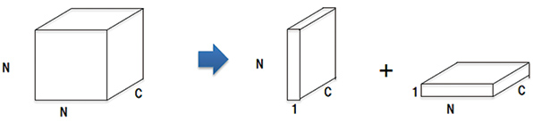
For the convolution operation, the computation amount increases in proportion to kernel size, and thus a higher speed can be obtained as the kernel size becomes smaller. On the other hand, for CNN, the effect equivalent to a convolutional layer of a larger-size kernel can be obtained by using multiple convolutional layers of a smaller size10). Therefore, we will shorten the overall computational time by dividing the convolutional layer with a kernel size of NxNxC into the two stages comprising the 1xNxC and the Nx1xC stages. (Fig. 5)
5.3 Fixed-point representation and utilization of parallel operation instruction
Convolution is a product-sum operation of floating-point data rows. On the other hand, for the CPU to be adopted for the image sensor, it is possible to use the single instruction multiple data (SIMD) that executes the product-sum operation of multiple data in parallel. In addition, SIMD enables the execution of many more parallel operations as the number of bits that express the data. Referring to the convolution calculation, we will enable the execution of up to 32 parallel operations by realizing the 8-bit fixed-point representation of inputs and outputs.
6. Performance evaluation
We applied the algorithm proposed in this paper to 466 inspection images (62 images for good products; 404 images for defective products) to evaluate performance. The precision of the conventional method used for comparison was calculated by optimizing the popular filters, including contrast enhancement and edge detection incorporated into the image sensor, for each object, thereby extracting the defect regions. Note, however, that the images used for evaluation were images wherein the imaging environment and imaging objects were different from the learning images adopted in this paper.
Table 2 shows the results of the performance evaluation. The category “false positive” shows incorrect detection from good product images and “false negative” shows non-detection of defective product images.
| false negative | false positive | |
|---|---|---|
| Conventional Method | 3.2% | 6.7% |
| Proposed Method | 0.9% | 3.4% |
Both results of false positive and false negative of the proposed method revealed higher precision. In addition, while the conventional method required the selection of multiple filters and adjustment of several parameters for each object, the parameters that required adjustments for using the proposed method were only threshold values for the feature map and a reduction in time and effort for the adjustment work at production site could be expected.
Figures 6 and 7 show the extraction result of the defect regions from using the proposed algorithm. The first row of the figure shows the input images, the second row shows the results of the extraction of defect regions from the input images using the conventional method incorporated into the image sensor for comparison. The final third row shows the extraction results of defect regions using the proposed algorithm. Fig. 6 shows the results of the case where images contain a pattern similar to the learning image, and Fig. 6(a) shows the object wherein the satin-finished aluminum is scratched. The width of the scratch of approx. 4 pixels was sufficiently fine for the resolution of approx. 2000×2000 of the input image where the contrast ratio was low, and processing with the conventional method was unable to extract the scratch at all. On the other hand, the processing result of the proposed algorithm was able to extract the scratched region that was not possible with the conventional method, and it ignored the shades of lighting showing a much greater salient contrast ratio on the image regions adjacent to the scratched regions. Fig. 6(b) shows a plastic film with stains on it. The film has fine hairlines, and when the image is processed with the conventional method, noise derived from the hairlines is widespread in the work. In contrast, the processing result with the proposed algorithm reveals that the defect regions could be extracted more clearly without being affected by the hairlines.
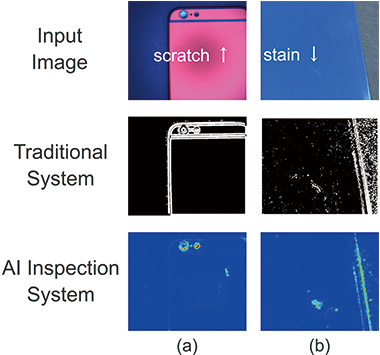
Fig. 7 shows the output results for objects when there were many differences from the learning image and there was information on the background region. Fig. 7(a) shows the images wherein a cracks is generated on the ferrite core, and an image that contained that type of information did not exist in the learning image. When processing with the conventional method was applied to this image, though extraction of cracked regions could be done, the shapes of the ferrite core and edges derived from the surface roughness were extracted as well. On the other hand, the processing result with the proposed algorithm revealed that only the cracked regions were output as the defect regions. Fig. 7(b) shows the image wherein dust exists on the wooden smartphone cover. The learning images did not include images of wooden objects, and the patterns wherein dust was included as defects did not exist because such patterns were not the targets in the present development. When processing with the conventional method was applied to this object, not only the dust, but also the wood patterned parts were extracted with similar intensity. On the other hand, treatment with the proposed algorithm revealed that, though learning of wood patterns and dust had not been made, the dust could be output as defects with the wood patterns ignored.
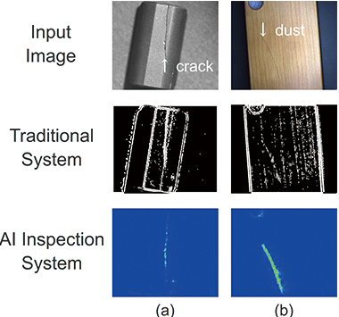
The results revealed that, while the algorithm proposed in this paper was of the pre-learning type, it had the ability to respond to unknown patterns that did not exist in the learning images.
7. Conclusion
In this paper, we proposed a pre-training type defect-detection algorithm that could handle a variety of objects and defect types. Through the proposed method, we verified that the algorithm could also handle objects and defects with unknown patterns.
For future prospects, we are examining the combined use with more complex technologies for inputs (lighting, imaging), driving technologies of robots, and online and additional learning to handle objects with more complex designs.
References
- 1)
- Maeda, H.; Sekimoto, Y.; Seto, T.; Kashiyama, T.; Omata, H.: Road damage detection using deep neural networks with images captured through a smartphone. arXiv:1801.09454, https://arxiv.org/abs/1801.09454, (accessed 2018-8-1).
- 2)
- Zhou, B.; Khosla, A.; Lapedriza, A.; Oliva, A.; Torralba, A. Learning Deep Features for Discriminative Localization. CVPR. 2016.
- 3)
- de Souza, C. R.; Gaidon, A.; Cabon, Y.; Peña, A. M. L. Procedural Generation of Videos to Train Deep Action Recognition Networks. CVPR. 2017.
- 4)
- Shrivastava, A.; Pfister, T.; Tuzel, O.; Susskind, J.; Wang, W.; Webb, R. Learning from Simulated and Unsupervised Images through Adversarial Training. CVPR. 2017.
- 5)
- He, K.; Zhang, X.; Ren, S.; Sun, J. Deep Residual Learning for Image Recognition. CVPR. 2016.
- 6)
- Szegedy, C.; Vanhoucke, V.; Ioffe, S.; Shlens, J.; Wojna, Z. Rethinking the Inception Architecture for Computer Vision. CVPR. 2016.
- 7)
- Xiang, W.; Zhang, D.-Q.; Yu, H., Athitsos, V. Context-Aware Single-Shot Detector, arXiv:1707.08682, https://arxiv.org/abs/1707.08682, (accessed 2018-8-1).
- 8)
- Liu, S.; Huang, D.; Wang, Y. Receptive Field Block Net for Accurate and Fast Object Detection. ECCV. 2018.
- 9)
- Sandler, M.; Howard, A.; Zhu, M.; Zhmoginov, A.; Chen, L.-C. MobileNetV2: Inverted Residuals and Linear Bottlenecks. arXiv: 1801.04381, https://arxiv.org/abs/1801.04381, (accessed 2018-8-1).
- 10)
- Simonyan, A. Z. Very Deep Convolutional Networks for Largescale Image Recognition. ICLR. 2015.
The names of products in the text may be trademarks of each company.