A Compensator that Negate the Influence of Grid Impedance based on Frequency Sweep Estimation Technique

In order to reduce the volume and cost of the PCS (Power Conditioning System), miniaturization of AC reactors (ACL) of inverters has been studied. If the ACL impedance value becomes smaller than the Grid-impedance between PCS and Grid, it is pointed out that a controllability of PCS has a risk of unstable. However, trying to improve the stability of control design, there will be a concern that the CPU calculation amount will increase. In this paper, we propose a control method that PCS itself estimates Grid-impedance with a small amount of calculation amount and set optimal control parameters as well. This control system is able to secure the stability according to the Grid-impedance after PCS installation, and further achieve a miniaturization of the ACL. As a result, it can contribute to downsizing and low cost of the entire PCS.

1. Introduction

1.1 The significance of spreading the use of renewable energy

In modern society, which relies on electronics, electricity is an essential source of energy. However, according to a survey conducted by the International Energy Agency (IEA), electricity generated from coal, natural gas and petroleum accounted for 81.4% of global power generation in 2015, meaning the global power generation is dependent on exhaustible resources ¹⁾. If this power generation continues, there is concern that global power generation that can meet the demand of society cannot be sustained. To solve this issue, the use of renewable energy has been taken into consideration. Although the high introduction cost of renewable energy had conventionally prevented its widespread use, introduction costs have been reduced as a result of improvement in efficiency and the downsizing of electric power converters. To realize a sustainable society, it is necessary promote the use of renewable energy through further cost reduction hereafter.

1.2 The role and issue with PCS

We are offering a PCS (Power Conditioning System) focusing on photovoltaic power generation as renewable energy. A PCS is a system that converts electricity generated by photovoltaic cells into AC power used in a grid power network for interconnection. Fig. 1 shows the external appearance of the PCS for photovoltaic power generation.

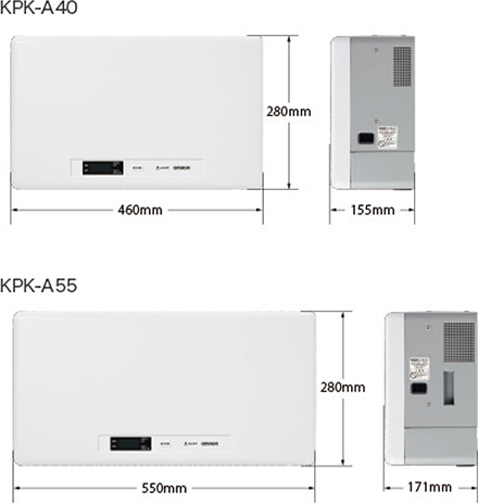
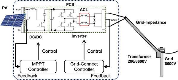
Fig. 2 shows the schematic view of a PCS with photovoltaic cells connected. The PCS consists of the following two electric converters: a DC/DC converter in the preceding stage and an inverter in the subsequent stage. The converter in the preceding stage controls the input power from the photovoltaic cells to constantly maximize it through the Maximum Power Point Tracking Control and feeds it to the inverter in the subsequent stage. The inverter in the subsequent stage converts DC power into AC power and feeds the power to the grid network while tracking grid variations through the Grid-Connect Control.
Among the parts which construct these electric converters, the reactor makes up a significant proportion of the cost and volume. In particular, downsizing the AC reactor (hereinafter referred to as “ACL”) that is used for the LC filter of the inverter leads to downsizing and cost reduction of the entire PCS.
However, when ACL is downsized, it has to face a problem that Grid-Connect Control becomes unstable due to current resonance of reactance components ( ) of conductor’s impedance (Grid-impedance) between PCS, and either ACL, LC filter capacitor (ACC), or Grid. The larger becomes relative to the ACL inductance value, the lower the resonance frequency of the current resonance and the higher the resonance gain becomes. If is small enough, there is no problem because the resonance frequency becomes much higher than the control frequency. On the other hand, if is large, the gain margin becomes insufficient and the stability is reduced because the gain increases owing to resonance in the frequency range where the phase is rotated by 180 degrees or more. To address this, the downsizing of the ACL was limited in the past because an ACL inductance value which was high enough for the estimated value set.

1.3 The position of previous studies and this paper

The suppression of resonance using a control software is being considered as the method of downsizing the ACL.

Among previous studies, there are documents ^{2) – 4)} reported cases where robust control such as H ∞ control and LQG (Linear-Quadratic-Gaussian) controllers are used as the methods of ensuring stability without estimating the grid impedance. However, since the computing load of the CPU becomes very high in such cases, these methods are not practical for PCS.
Methods of designing a controller based on the estimated grid impedance have also been suggested. The literature ⁵⁾ suggested the injection of harmonics into the output voltage to estimate the absolute impedance value based on the amplitude variation. However, this method requires the mounting of several SOGIs (Second Order Generalized Integrators) with a high computing load to enhance the accuracy. The literature ⁶⁾ suggested the method of estimating the impedance from the output voltage regulation when active and inactive powers were varied. However, this method requires the building of a control system for operating active and reactive powers independently, and there is concern that the computing load may increase.
This paper describes a method which negates the influence of grid impedance so that even a small ACL becomes stable. Since the compensator optimizes the compensator parameter based on the grid impedance value estimated according to a computing method simpler than the one used in previous studies, there is no need to design ACLs based on the maximum value which is estimated for the grid impedance and varies depending on the place of installation. Therefore, the further downsizing of ACL can be realized.
Chapter 2 describes the influence and issues with grid impedance made when a conventional control system is built. Chapter 3 shows how to estimate grid impedance and design the compensator. Chapter 4 presents the effectiveness of the suggested method based on the simulation results, and Chapter 5 gives a summary of this paper.

2. The influence of grid impedance on Grid-Connect Control

2.1 The configuration of Grid-Connect Control

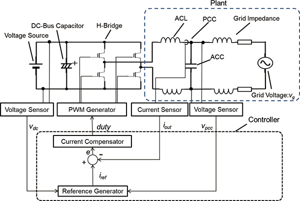
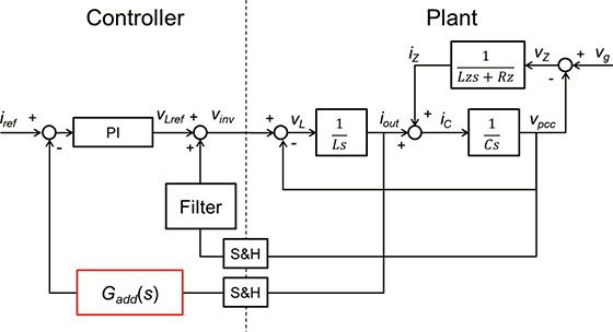
Fig. 3 shows the complete view of the Grid-Connect Control of the inverter. The Grid-Connect Control is made up of a command value generation section which generates a current command value synchronized with the AC voltage phase of the Point of Common Coupling (PCC), a current controller which controls output current, and a controlled object consisting of the inverter circuit, grid impedance and grid voltage. The control system manipulates the inverter modulation factor based on the duty width of the PWM signal to control output current.

2.2 Unstable current control caused by grid impedance

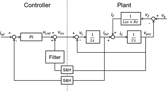
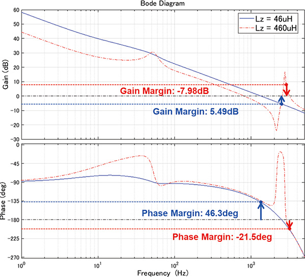
To determine the stability of the current control system on Matlab/Simulink, we modeled the control system and controlled object. Fig. 4 shows the block diagram of the modeled current control system. Fig. 5 shows the Bode diagram of the open loop transfer functions of the current control system. The parameters of respective conditions are as shown in Table 1.
The graphs indicated with solid lines in Fig. 5 show the open loop transfer functions when is 46 μH and is 38 mΩ. The stability of the control system is evaluated based on the gain and phase margins. The gain margin represents a phase value at the point where the phase is rotated by 180 degrees. Since the resonance peak occurs at a frequency higher than the control band (half of the PWM carrier frequency) because is small enough, the stability is not impaired. In this example, the stability is secured because the gain margin and phase margin are 5.49 dB and 42 degrees, respectively. In addition, the bandwidth exceeds 1 kHz, which is higher than commercial frequency and ensures sufficient responsiveness.
The graphs indicated with dashed lines in Fig. 5 show the open loop transfer function when is 460 μH and is 380 mΩ. Since the resonance point became lower than the carrier frequency owing to increased , an antiresonance is observed at around 3 kHz. An increase in gain occurred in the range where the phase is −180 degrees or smaller, leading to unstable control. The gain margin and phase margin were −7.98 dB and −21.5 degrees, respectively. To improve this situation only through PI control, the bandwidth needs to be reduced, which may result in a deterioration in the high-frequency wave responsiveness, distortion of output waveform and impossibility of satisfying the harmonic regulation.

Table 1. Parameters used when drawing the open loop transfer functions

Condition No.	1	2
Grid voltage	202 Vrms	202 Vrms
Grid voltage frequency	60 Hz	60 Hz
Imaginary part of grid impedance:	46 μH	460 μH
Real part of grid impedance:	38 mΩ	380 mΩ
AC reactor	720 μH	720 μH
AC capacitor	12 μH	12 μH
PWM carrier frequency	10 kHz	10 kHz
P gain of PI controller	6.48	6.48
I gain of PI controller	454.4	454.4

3. Design of the control compensator

3.1 How to estimate grid impedance

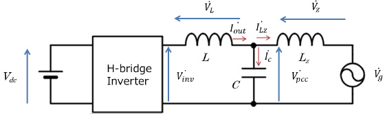
Fig. 6 shows the equivalent circuit of the controlled object. In this figure and the equation to be described below, the inductance value of the ACL and the capacitance value of the ACC are expressed as and , respectively. Supposing is dominant in the grid impedance, is omitted.
The grid connection point voltage shown in Fig. 6 is represented by the equation (1).

• (1)

In the equation (1), reaches a local maximum value when the following equation is satisfied:

• (2)

Where, is represented by the following equation (However, 2 = ).

• (3)

Fig. 7 shows the equation (3) graphically.

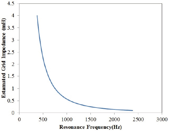
Among the variables shown in the equation (3), and are already known because they are set by the designer. Therefore, if a resonance frequency is estimated and substituted into of the equation (3) in some way, it becomes possible to estimate an unknown parameter . If a small signal disturbance is introduced into the command value of the current control system, a response appears in in the form shown in the equation (1). fc can be estimated by sweeping the frequency of the small-signal disturbance to search for the condition which maximizes .
In addition, although the output filter of the inverter shows an example of LC filter this time, can be derived also in the case of LCL filter. Since the result obtained from the equation (3) is the sum of the ACL inductance values and on the LCL filter system side, deducting the known enables to be derived as well.

3.2 The configuration and algorithm of the suggested system

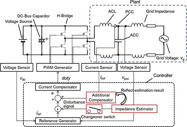
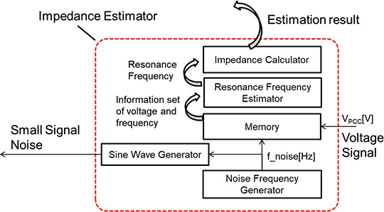
Fig. 8 shows the configuration of the entire system suggested, which was created by adding the impedance estimation section, the impedance suppression compensator section and the configuration changeover switch to the configuration shown in Fig. 3. Fig. 9 shows the internal configuration of the added impedance estimation section.
The procedure for estimating impedance is as follows: Activate the control system of the PCS to output the electric voltage interconnected to the system voltage. In this case, the electric current which is output by the PCS is zero, and the electric voltage which is completely synchronized with the system is output. Next, substitute the initial value into the disturbance frequency which is superimposed on the disturbance frequency generation section shown in Fig. 9. This creates a disturbance signal from the sine wave disturbance generation section, and turning on the configuration changeover section superimposes the disturbance signal on the command value and the disturbance voltage on . In this case, memorize the maximum voltage of on which the disturbance is superimposed and which is currently output in the memory section as a pair, and add to the disturbance frequency to update. Repeat this procedure until the disturbance frequency reaches the maximum value .
Finally, turn off the configuration changeover section to stop the disturbance superimposition. Extract a pair which reached the maximum voltage from among values memorized, and set value in this case as the resonance frequency fc. Substituting this resonance frequency fc into f of the equation (3) enables the Grid-impedance to be obtained.
The sweep range values and can be determined using the equation (3) if the designer specifies the range of to be estimated after setting and values.
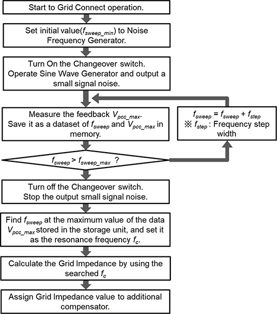
Fig. 10 shows the flow chart of a sequence of operations.

3.3 Design of the compensator

The compensator is designed based on the estimated Grid-impedance. The resonance frequency of the current can be determined based on the equivalent circuit model shown in Fig. 6 as represented by the equation (4).

• (4)

It turns out that an increase in resonance gain which causes unstable factors occurs in obtained by this equation. Therefore, a compensator (s) which suppresses the gain in the bandwidth is additionally mounted. The transfer function of the compensator is represented by the equation (5), which is a notch filter that reduces the gain of a specific frequency band.

• (5)

4. Simulation results

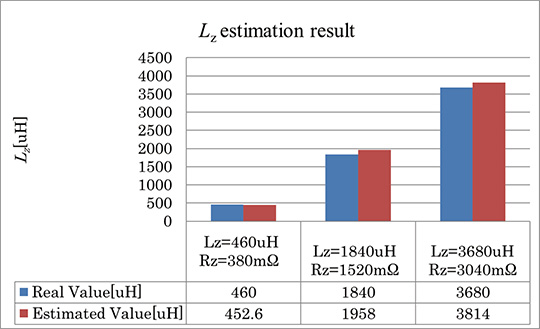
We implemented the algorithm for estimating the Grid-impedance on Matlab/Simulink, and to measure its accuracy, we estimated the impedance in combination with the circuit simulator implemented on Simscape. We estimated the Grid-impedance values and under three conditions (one time, four times and eight times) based on the values of condition 2 shown in Table 1. Fig. 11 shows the simulation results. Under respective conditions, the estimation values close to true values were obtained.

Next, we designed the compensator based on the estimated impedance to confirm whether the control stability would be improved or not. For the values and , we used those in condition 1 shown in Table 1. If the estimation results when is 460 μH and is 380 mΩ is substituted into the equation (5), the following equation can be obtained.

• (6)

To perform the current control system stability determination, we built the block diagram shown in Fig. 12 on Simulink and substituted the result of the equation (6) into the (s) block.
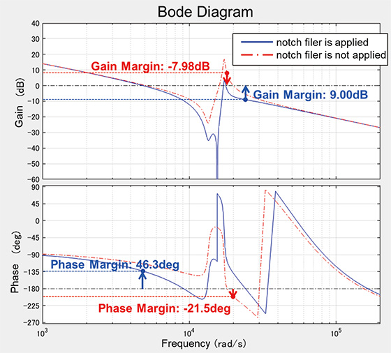
Fig. 13 shows the open loop transfer functions of the current control system. The blue solid lines show the condition where the compensator (s) is added, and the red dashed lines show the condition where no compensator was added (identical to the graph indicated with a dashed line in Fig. 5). We can find that adding the compensator achieved stable control. The gain margin, phase margin and bandwidth were 9.0 dB, 46.3 degrees and 769 Hz, respectively. Although the bandwidth was narrower than the condition where Lz was 46 μH shown in Fig. 5, since the gain of 20 dB or higher was secured at commercial frequency, we consider it has little effect on waveform distortion.

5. Summary

In this paper, we showed an example of designing a compensator based on the method of estimating the Grid-impedance using the frequency sweep method and impedance for LC type and LCL type output filters of the PCS inverter. Designing the compensator in conformity with the Grid-impedance obtained after installing the PCS enables the downsizing of the ACL without impairing the stability.
Since this method enables enhancement of the stability of the control system simply by adding the impedance estimation section, the impedance suppression compensator section and one secondary compensator to the conventional configuration, it is possible to cope with the disadvantage of downsizing the ACL.

References

1)

International Energy Agency. “Key World Energy Statistics 2017”. https://www.iea.org/publications/freepublications/publication/KeyWorld2017.pdf, (accessed 20180219).

2)

J. Chen, F. Yang and Q. Han. Model-Free Predictive H∞ Control for Grid-Connected Solar Power Generation Systems. IEEE Transactions on Control Systems Technology. 2014, vol. 22, Issue 5, p. 2039-2047, doi:10.1109/TCST.2013.2292879. https://ieeexplore.ieee.org/document/6720111

3)

V. P. Singh, S. R. Mohanty, N. Kishor and P. K. Ray. Robust H-infinity load frequency control in hybrid distributed generation system. International Journal of Electrical Power & Energy Systems. 2013, vol. 46, p. 294-305, https://www.sciencedirect.com/science/article/pii/S0142061512005789

4)

F. Huerta, D. Pizarro and S. Cobreces, LQG Servo Controller for the Current Control of LCL Grid-Connected Voltage-Source Converters. IEEE Transactions on Industrial Electronics. 2011, vol. 59, Issue 11, p. 4272-4284, doi:10.1109/TIE.2011.2179273. https://ieeexplore.ieee.org/abstract/document/6099608

5)

J. Moriano, V. Bermejo, E. Bueno, M.Rizo and A. Rodriguez. A Novel Approach to the Grid Inductance Estimation based on Second Order Generalized Integrators. ECCE Cincinnati. 2017, p. 1794-1801, doi:10.1109/ECCE.2017.8096012. https://ieeexplore.ieee.org/document/8096012

6)

M. Ciobotaru, R. Teodorescu, P. Rodriguez, A. Timbus and F. Blaabjerg. Online grid impedance estimation for single-phase gridconnected systems using PQ variations. Power Electronics Specialists Conference. 2007, p. 2306–2312, doi:10.1109/PESC.2007.4342370. https://ieeexplore.ieee.org/abstract/document/4342370

The names of products in the text may be trademarks of each company.