Consideration of Improving Machining Accuracy by Disturbance Correction Using Machine Learning
- AI technology
- PLC
- Feedforward control
- Disturbance correction
- Servo press machine
At the manufacturing site, it is necessary to improve processing accuracy while maintaining and improving productivity. As a result, in recent years, variations and fluctuations in materials and machines at manufacturing sites cannot be ignored. At the manufacturing site, in order to suppress such disturbance effects, various control methods are devised, and production equipment is adjusted by field workers to prevent deterioration of processing accuracy.
Generally, feedback and feedforward control is used to suppress the influence of disturbance, but the effect of feedback control may be insufficient because the correction is performed after the influence of disturbance appears. Furthermore, in the case of feedforward control that performs disturbance correction using a mathematical model, there is a problem that the prediction error becomes large and the machining accuracy deteriorates in the controlled object that depends on the usage environment. Therefore, in this paper, we propose a method for improving processing accuracy by disturbance correction using machine learning. Using the proposed method of bottom dead center correction control of the servo press, it was confirmed that the machining accuracy was improved so that the mean squared error (MSE) was 1/6 of the conventional method.
1. Introduction
At the manufacturing site, it is necessary to improve machining accuracy while maintaining and improving productivity.
As a result, in recent years, the influence of disturbances, such as variations and fluctuations in the materials and machines at manufacturing sites (hereinafter referred to as “2M fluctuations”), cannot be ignored. For example, in the press working, the machined accuracy is regarded particularly important as a quality characteristic. Machining accuracy in presswork is mainly affected by variations in material thickness and changes in the state of the manufacturing equipment, and when machining accuracy deteriorates, the machining accuracy is improved by adjusting the manufacturing equipment1). In general, feedback and feedforward control is used for suppressing the influence of disturbance. However, because of the principle of feedback control that makes corrections based on the results of the given operation amount, correction is possible only after the appearance of external disturbances, which leads to the production of defective products. Feedforward control also requires an appropriate amount of correction for performing a correction to reduce the influence of disturbances before they appear. However, if a mathematical model is applied for disturbance correction, in other words, application to a control target that depends on the usage environment, such as the 2M fluctuations, may result in a large prediction error and lead to deterioration of machining accuracy.
From such a background, the methods have been considered to prevent the deterioration of product machining accuracy by correction through iterative learning control to suppress the influence of disturbances2). Iterative learning control is a method that can improve performance by repeating trials in cases where similar conditions are repeated. However, disturbance correction is difficult because, in principle, the learning does not proceed for disturbances that fluctuate over time, such as the equipment degradation or temperature rises due to processing.
Hence, in this paper, we propose a disturbance correction method using machine learning that has overcome the problems of conventional methods. The proposed method can prevent the deterioration of product machining accuracy due to 2M fluctuations, including the fluctuating disturbances over time.
In this experiment, the proposed method in our machine automation controller3) with our built-in AI (hereinafter referred to as AI controller) was implemented and the effectiveness was verified. In an AI controller, the control of manufacturing equipment and AI technology coexist in a machine automation controller, with functions for collecting time series data, calculating feature quantities and detecting outliers.
2. Subjects
A feedback control system, in which multiple disturbances d of the 2M fluctuations are applied to a tool/workpiece system in the machining zone, is shown in Fig. 1. The disturbance in this paper includes those that fluctuate over time that cannot be handled by conventional methods as well. The Setting Value s of the processing machine is generated from the Quality Characteristic Standard Value qr, the Quality Characteristic Value q is fed back, and the Target Value o is output from the Target Value Generation. The controller controls the mechanism by outputting the Operation Amount u from the Target Value o and the Control Amount y and processes the workpiece through the tools. In the case of a feedback control system, the target value is adjusted automatically or manually using Quality Characteristic Value q to achieve a control in which the variation of Quality Characteristic Value q is reduced. However, in a feedback control system, the Setting Value s is corrected after the influence of the disturbance appears in the Quality Characteristic Value q. Because of this, depending on the individual differences in the processed material or the differences in the operating environment, such as climate, season, date, and time whose conditions are difficult to maintain at a stable level, the appropriate corrections are not immediately made and good Quality Characteristic Value q is not obtained.

Hence, in this paper, a feed-forward control system is considered that corrects Setting Value s by using a corrector that uses Disturbance d of the 2M fluctuations applied to the Tool/Workpiece as an input and Correction Amount c as an output, as shown in Fig. 2.

The corrector is required to output an appropriate amount of Correction c that reduces the variation in Quality Characteristic Value q according to Disturbance d of the 2M fluctuations that may occur during manufacturing. However, since Disturbance d of the 2M fluctuations is highly dependent on the operating environment and fluctuates over time, it is difficult to apply the feed-forward control or the iterative learning control that uses a general mathematical model for correction of disturbances.
Hence, a method using machine learning for the easy design of a corrector, which is difficult in feed-forward control, is explained in the following paragraphs.
Additionally, it is obvious that if the disturbance is small enough, it will not affect the quality, but if it is extremely large, the correction by the control system will be impossible. Hence, in this paper, it is assumed that Disturbance d of the 2M fluctuations has a magnitude that can cause defective products and does not exceed the range assumed in the control system design.
3. Proposed Method
3.1 Corrector Configuration
The configuration of the corrector proposed as the method is shown in Fig. 3. The corrector consists of a feature quantity calculator and a predictor and has a configuration of predicting the appropriate Correction Amount c from the measured Disturbance d of 2M fluctuations.

The feature quantity calculation section measures Disturbance d of 2M fluctuations that affects the quality characteristic value with a sensor, and making it into the feature quantities, such as average values and maximum values. The predictor outputs Correction Amount c according to the feature quantity f using a prediction model with the supervised learning algorithm.
3.2 Corrector Structuring Procedure
The first step in structuring a corrector is to collect production data (Correction Amount c, Disturbance d of 2M fluctuations measured by sensors and Quality Characteristic Value q) using the conventional methods (setting by skilled operator, feedback control, etc.) The reason for collecting Quality Characteristic Value q in spite of not being used for control is complemented in the following: The collected data are not necessarily of the good products because it is based on conventional methods and may include data of defective products. Even if they are acquired from good products, there is a variation in quality characteristic values, and data close to the upper/lower limits of the standard are included as well. Therefore, if all of the collected data is used as training data, the prediction model will be the one that outputs a Correction Amount c that causes a large variation in Quality Characteristic Value q and no improvement in machining accuracy is expected. Hence, in the data preprocessing, the data set with the smallest variation in Quality Characteristic Value q is selected from the collected data for learning. For information, the learning of the predictor is conducted offline, and the generated prediction model and the calculation of Feature Quantity f selected during the data preprocessing is implemented in the controller.
- (1) Data Collection
Production data are collected including Quality Characteristic Standard Value qr, Quality Characteristic Value q, Disturbance d measured by the sensor and Correction Amount c determined by the conventional method during the manufacturing of product using the conventional method. - (2) Data Preprocessing
In this paper, a section in production equipment where a repetitive motion takes place is called a “frame.” Since the collected data is the time-series data, statistical feature quantities, such as average value and maximum value, are calculated per each specific section of the frame and are associated with the corresponding Correction Amount c to form a data set. To select the Feature Quantity f used in the feature calculation section, the causal analysis, the importance analysis, etc. are applicable. Remove data with Quality Characteristic Value q far off from Quality Characteristic Standard Value qr from the data set and divide the data into learning/evaluation data. For information, Quality Characteristic Standard Value qr and Quality Characteristic Value q are deleted from the data set because they will not be used in the subsequent processing. - (3) Learning of Predictor
Learn a regression model that predicts the Correction Amount c from Feature Quantity f. There are various methods for regression; in this paper, a machine learning algorithm, Dynamics Learning Tree (DLT)4) that can perform high speed prediction processing was used. - (4) Evaluation
The prediction accuracy was evaluated using the evaluation data and the performance of the prediction model has been evaluated.
Applying the corrector structured in accordance with the above procedure to a feed-forward control system in Fig. 2, the Correction Amount c, which cancels the effect of Disturbance d, is appropriately determined to enable disturbance suppression control.
4. Experiment
4.1 Subject of Experiment
In this experiment, we implemented this method on an AI controller and connected it to the servo press machine ZENFormer nano by the Hoden Seimitsu Kako Kenkyusho Co., Ltd., and performed pressing with the bottom dead center position control.
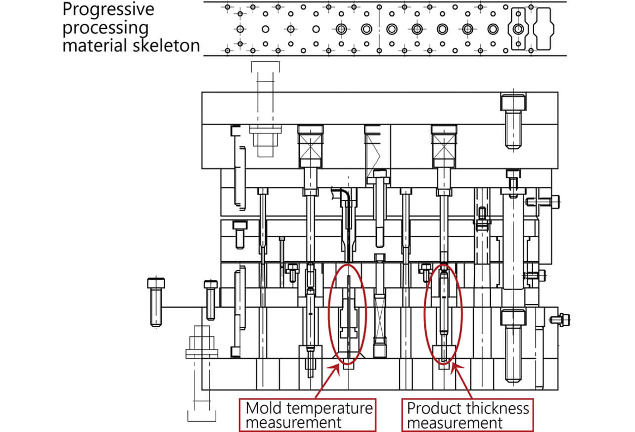
The ZENFormer nano is a four-axis direct-drive servo press that uses a ball screw in its force-increasing mechanism, allowing the slide surface control in increment of micrometer units. The die layout is shown in Fig. 4. A servo press machine is equipped with sensors that measure various conditions, such as die temperature and product thickness. In the progressive processing, material flows from left to right, where material thickness is assumed to be measured in advance when the rolls are changed.
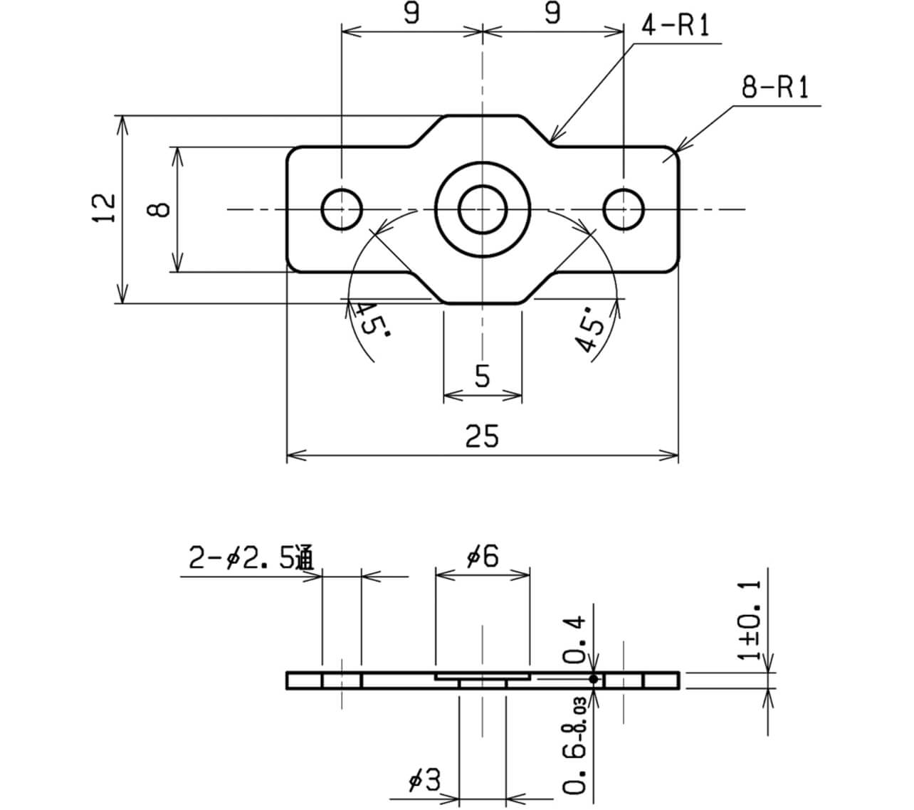
SPCC-SD, a common cold-rolled steel strip of t 1.00±0.05 [mm] and W 32.0±0.20 [mm], used for manufacturing a flange shown in Fig. 5, and pressed it so that the thickness of the center indentation is 0.6±0.01 [mm].
Furthermore, the correspondence with the control system shown in Figs. 1 and 2, and the common conditions and the setting values in this experiment are shown in Table 1.
| Category | Item | Condition/Setting |
|---|---|---|
| Quality Characteristic Standard Value: qr | Target Product Thickness | 0.6±0.01 [mm] |
| Quality Characteristic Value: q | Product Thickness | ― |
| Setting: s | BDC Setting | 84.200 [mm] |
| Correction Amount: c | BDC Correction Amount | ― |
| Controlling Amount: y | Slider Position | ― |
| Disturbance: d | Die Temperature, Material Thickness | ― |
| ― | Forming Speed | 30 [mm/s] |
| ― | BDC Duration | 500 [ms] |
| ― | Ambient Temperature at Experiment Start | 20~20.9 [°C] |
4.2 Calculation of Correction Amount
In this experiment, machining accuracy and errors are compared by (a) manual correction in which a person plays the role of the corrector in Figure 1, (b) automatic correction using the method in Reference Literature 1), and (c) automatic correction using the proposed method.
- (a) Manual Correction (conventional method)
Periodically sample and measure the product thickness at four locations using a micrometer. When the average of the product thickness at four locations exceeds 0.6 ± 0.003 [mm], the operator manually sets the bottom dead center correction amount to the current correction amount ∓ 0.003 [mm]. - (b) Automatic Correction (conventional method)
The program automatically sets the bottom dead center correction amount to ∓0.003 [mm] of the current correction amount when the difference between the average product thickness and the target value for 100 consecutive shots exceeds ±0.003 [mm]. - (c) Proposed Method
Feature Quantity f is calculated from the die temperature and material thickness and the predictor calculates the bottom dead center correction amount for each shot. The die temperature is measured during the control, and it varies from shot to shot, but the material thickness is measured in advance for each roll, and it is assumed not to vary from shot to shot.
4.3 Structuring the Proposed Corrector
Follow 3.2 “Corrector Structuring Procedure” and collect production data under (b) Automatic Correction to structure the corrector. In this experiment, among the collected production data, the data of product thickness within 0.6±0.003 [mm] are used as the learning data. The average value of Disturbance d is used for the feature quantity calculation.
For information, the production data for structuring a corrector, in addition to the data shown in the experimental results, were collected from the multiple material rolls. The ranges of learning data are shown in Table 2.
| Item | Learning Data |
|---|---|
| Material Thickness [mm] | 0.9940~1.0182 |
| Die Temperature [°C] | 19.2~26.5 |
4.4 Experimental Results
The experimental results of 4,000 shots for each of (a) Manual Correction, (b) Automatic Correction, and (c) Proposed Method are explained.
- (1) Trend of Disturbances
The average material thicknesses for the experiment of each method are shown in Table 3. The standard of material roll thickness is 1.00±0.05 [mm]. Since the material rolls used for each method were different per experiment, the average material thicknesses were different as well.
| Item | (a) Manual Correction | (b) Automatic Correction | (c) Proposed Method |
|---|---|---|---|
| Average Material Thickness [mm] | 0.9996 | 0.9968 | 1.0061 |
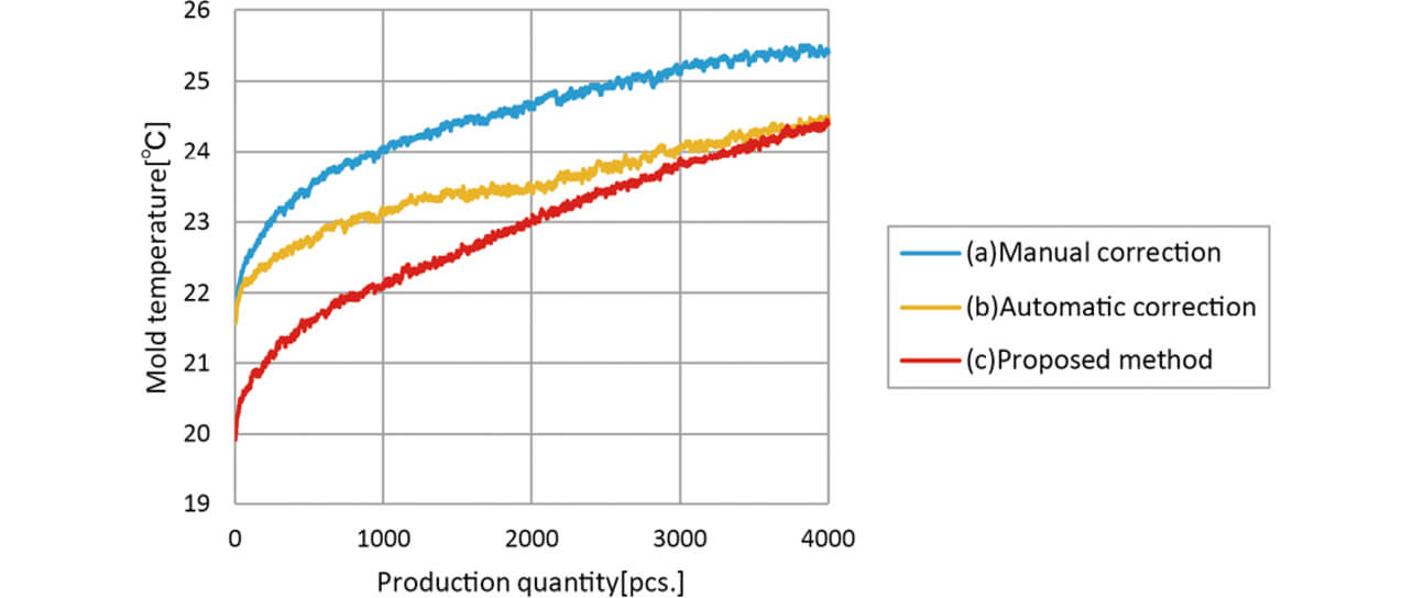
The die temperature fluctuations during the experiment of each method are shown in Fig. 6. In all cases, the temperature tends to rise with time, but due to the differences in date/time of experiment, etc., there are differences in the experiment start die temperatures and in the way the temperature rises.
- (2) Correction Result
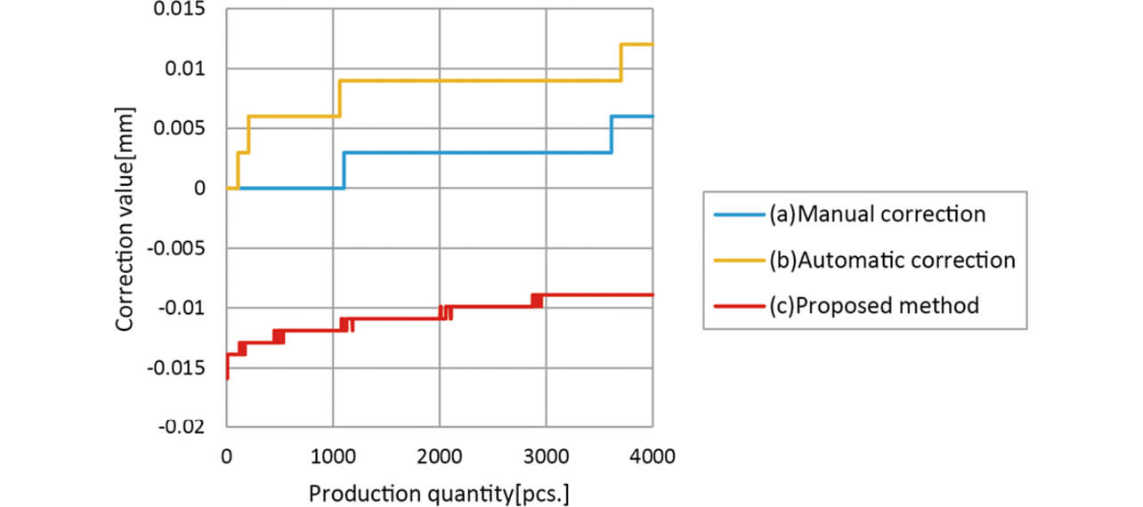
The amount of correction resulting from the execution of each correction method is shown in Figure 7. It is recognizable that, compared to (a) Manual Correction and (b) Automatic Correction, the amount of correction in (c) Proposed Method could more closely follow the variation of mold temperature than others. The initial difference in the amount of bottom dead center correction for each method reflects the material thickness and die temperature. In the conventional methods (a) and (b), the initial value was zero due to the delay of feedback, and it took more time to reach an appropriate correction amount than by the proposed method (c).
- (3) Comparison of Quality Characteristic Values
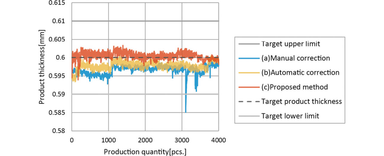
The results of measuring the product thickness, a quality characteristic value, by applying a relevant bottom dead center correction method are shown in Table 4 and Fig. 8, and the performances are compared and discussed in the below.
| Item | (a) Manual Correction | (b) Automatic Correction | (c) Proposed Method |
|---|---|---|---|
| Average [mm] | 0.5966 | 0.5978 | 0.6005 |
| Standard Deviation [mm] | 0.0012 | 0.0010 | 0.0008 |
| MSE [mm2] | 1.272×10⁻⁵ | 0.585×10⁻⁵ | 0.096×10⁻⁵ |
| Process Capability Index (Cpk) | 1.89 | 2.56 | 3.75 |
- (a) Manual Correction
The process capability index was 1.89, which was sufficient for the process capability, but the product thickness at the initial stage of production was at the lower limit side of the target and resulted in the biased product thickness from the target product thickness due to correction based on infrequent sampling. Sudden variations in product thickness that exceeds the lower target limit are considered to be due to the influence of temporary dust bites or the lubrication conditions, since there is no extremely large change in material thickness or die temperature. - (b) Automatic Correction
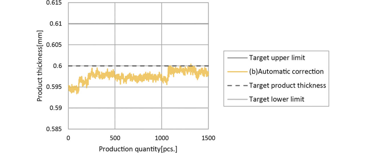
The product thickness around the time of experiment start is shown in Fig. 9. The machining accuracy was higher than (a) manual correction, but the product thickness was biased in a similar manner. The extended time required to converge to the target product thickness is considered due to the method using the average product thickness for 100 shots as the correction amount. - (c) Proposed Method
Compared to (b) the automatic correction, the average product thickness was improved by 0.0017 [mm] and the standard deviation that indicates the variation in product thickness was improved by 0.0002 [mm]. In addition, the results shows the distribution around the target product thickness as the center from the start of production, which suggests that the influence of die temperature and the change of material rolls are appropriately reflected in the correction amount. As a result, the product thickness was close to the target product thickness of 0.6 [mm], and the MSE was improved to 1/6 compared to (b) Automatic Correction.
5. Conclusions
In this paper, we proposed a disturbance correction method using machine learning to predict the amount of correction for disturbances that cannot be adequately suppressed by conventional methods. This method was applied to the press working using the bottom dead center position control of the servo press machine, and the improved working accuracy of MSE to 1/6 of the conventional automatic correction was confirmed.
This method uses machine learning to predict the appropriate correction amount for the trend of 2M fluctuations dependent on the operating environment, and has shown that it can control with higher accuracy than conventional methods. In this experiment, the improvement effect on the process capability was obtained by applying this method to the processes that already had a sufficient process capability with the conventional method. It is also expected that the manufacturing of high-precision products with stricter dimensional tolerances than before will be possible.
In this experiment, only two disturbances, material thickness and die temperature, were considered: in machine learning, in general, there are issues of the increased amount of required learning data as the number of variables increases and “the curse of dimensionality”, which makes it difficult to structure a prediction model. For this reason, it is considered necessary to conduct future experiments on the objects that have more number of variable factors. Furthermore, the verification will be continued on the versatility, stability, and safety of this method, through the simulations and evaluations by implementing in other objects.
Acknowledgments
We would like to express our gratitude to the cooperation given to our experiments by the members of the Industrial Machinery Business Division of the HODEN SEIMITSU KAKO KENKYUSHO CO., LTD.
References
- 1)
- C. Murata, “Sensing Technology for Presses and Dies - Mechanisms of Press Working Seen from Servo-Presses and Dies,” Materials Process Technol., vol. 58, no. 9, pp. 17-23, 2017.
- 2)
- T. Fujii, Y. Ueyama, and Y. Abe, “A Study on Correction of Bottom Dead Center of Servo Press Machine by Iterative Learning Control,” 2018 IEE-Japan Industry Applications Soc. Conf. Lecture Papers, Aug. 28, 2018, pp. 19-22.
- 3)
- T. Mioki and J. Deki, “Development of AI-Equipped Machine Automation Controller (1),” OMRON TECHNICS, vol. 51, no. 1, pp. 39-44, 2019.
- 4)
- A. Numakura, S. Kato, K. Sato, T. Tomizawa, T. Miyoshi, T. Akashi and K. C. Hae, “Dynamic Learning Tree - Multi-Layered Learning for Continuous Dynamics,” in The 77 th National Convention of IPS, vol. 2015, no. 1, pp. 993-994.
The names of products in the text may be trademarks of each company.


