


A Proposal for a Causal Analysis Method for Product Defect by Integrating Control Program Analysis and Data Analysis
- Program Slicing
- Mutual Information
- Causal Analysis
- Directed Graph
- PLC
In recent years with the trend toward IoT, there has been an increase in cases of causal analysis for product defects in the Factory Automation (FA) field. However, a conventional method is not effective because the collected data has low independence by multiple processes and synchronous control. To solve the issue, we focus on a PLC control program that has information of them. In this paper, we propose a method to integrate knowledge from the PLC control program by applying a program slicing technique into data analysis. In addition, we show the method is effective for cases that do not work by the conventional one with an automatic packaging machine.
1. Introduction
Following the recent widespread use of IoT (Internet of Things), there have been increasing cases of collecting sensing or control data from shop floors in the FA field for product defect factor analysis1,2). However, as can be seen from the fact that Ishikawa diagrams3) are used to organize domain knowledge information in the field of quality control, the analysis of collected data alone cannot easily enable the identification of appropriate factors.
Traditional assumptions have it that factor analysis based on decision tree importance values serves well as an approach to addressing a defect or trouble that may be encountered4,5). However, a total reliance on the decision tree importance calculated from control data will often result in selecting too many potential factors to reach the true cause. The cause is that the only data available is the synchronized data of multiple processes and low in stochastic independence.
In the FA field, mainly physical assembly or processing processes are automated to manage high production capacity and high-quality production at a high operating ratio, thereby improving the overall equipment efficiency defined as operating ratio ×performance ×quality 6). Therefore, FA control technologies are characterized primarily by multi-process parallelization for higher production capacity and high-precision synchronous control for higher quality. As a result, control data collected from shop floors are characterized by low independence because of the synchronous control of multiple processes.
Taking note of a PLC control program containing multi-processing and synchronous control information, we propose to extract knowledge information from the control program and integrate it into data analysis. Our proposed method uses a program slicing technique to merge a variable dependence graph generated from the PLC control program with a structural change graph generated from control data, thereby enhancing the independence of control data to improve the accuracy of factor estimation. What follows presents an experiment performed using an experimental packaging machine to demonstrate that our proposed method can identify event factors unidentifiable by the conventional method.
2. Conventional method and its problems
This section describes the behavior of the packaging machine, the targeted system, to explain the problem with control data of low stochastic independence due to multiple synchronized processes in a control system.
2.1 Targeted system
Fig. 1 shows the experimental packaging machine, which is the targeted system.
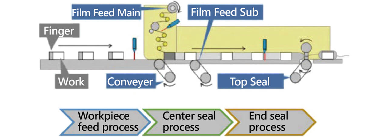
The targeted packaging machine is a horizontal pillow packaging machine used to package products with resin-made film. Its PLC synchronously controls four servomotors to automate the packaging process. This packaging machine consists of three processes, a workpiece feed process with fingers feeding out workpieces, a center seal process, and an end seal process to pack workpieces in pillow-shaped packages. The four servomotors are controlled as a conveyor shaft for workpiece feed, film feed shafts 1 and 2 for the center seal process, and a top seal shaft for the end seal process, respectively. Their respective torque, velocity, and position signals are collected as control data. Incidentally, product defect factor analysis based on these control data adds the benefit of making it unnecessary to retrofit sensors to the machine.
2.2 Conventional method
A typical conventional factor identification method consists of the following steps:
- 1. Calculate feature quantities from control data.
- 2. Compute the decision tree importance from all the feature quantities.
- 3. Identify the condition corresponding to the highest-importance feature quantity as the factor.
Fig. 2 shows a conceptual diagram of feature quantity calculation from control data:
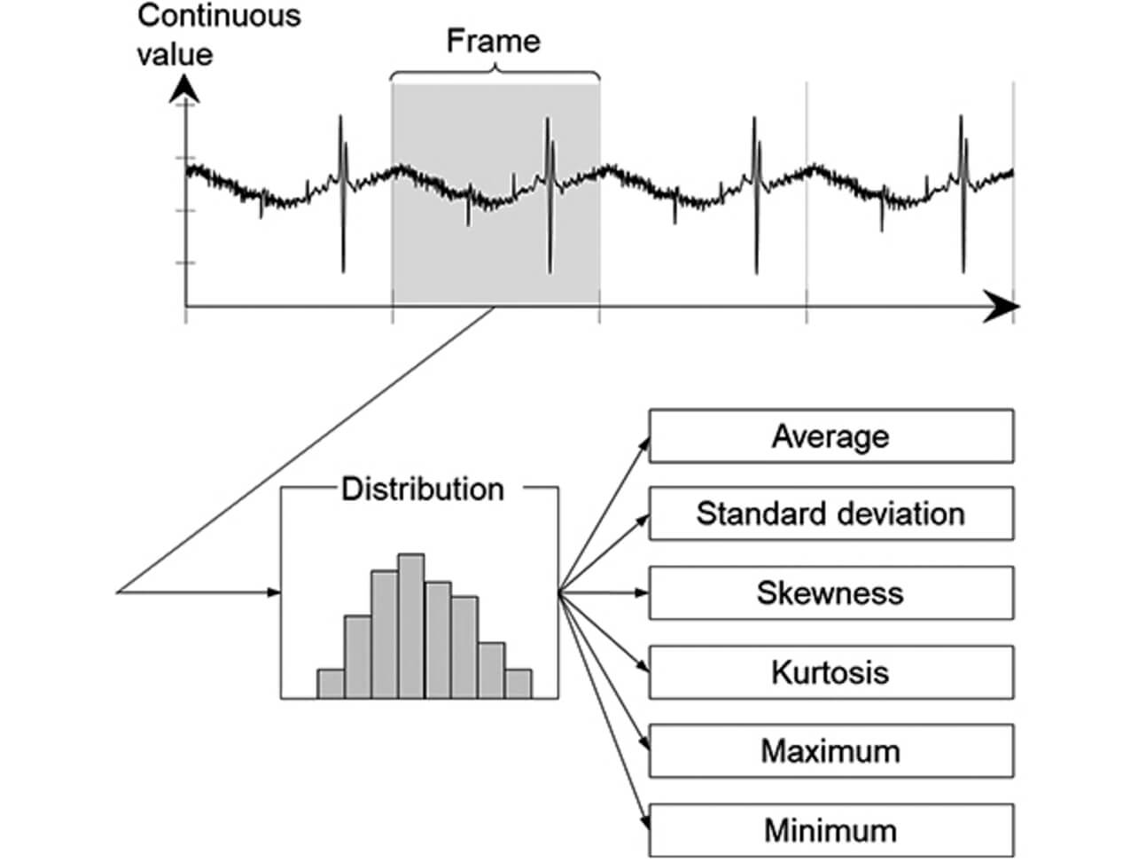
For the purposes here, collected control data are divided into manufacturing cycle units called “frames” to calculate multiple statistical quantities, such as mean value and standard deviation, as feature quantities. In the case of the packaging machine above, the frame is the unit for packaging workpieces.
Next, for all the feature quantities, their importance values are calculated to select feature quantities with higher importance values. The conventional practice has been to identify conditions corresponding to these feature quantities as factors. A decision tree is a machine learning method that performs classification or regression using a tree structure. What is meant here by “importance” is the decrease in the Gini coefficient before and after a normal/anomalous determination based on each feature quantity. The greater the value is, the better a feature quantity serves as a normal/anomalous discriminant variable.
2.3 Problem with the conventional method
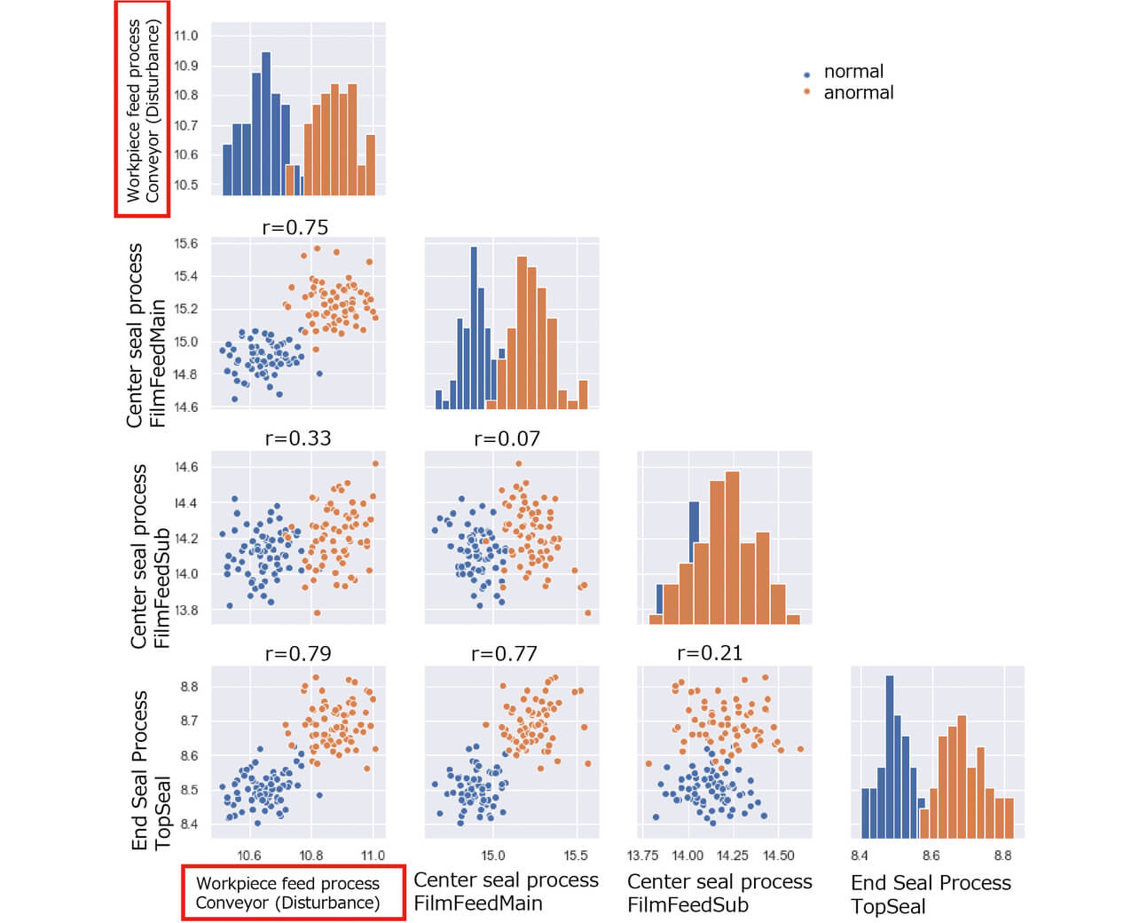
Fig. 3 shows a typical scatter diagram of feature quantity data used in the conventional method. The scatter diagram shows the relationship between normally packaged workpieces and those packaged during the application of disturbance as a quasi-anomaly to the conveyor shaft in terms of the torque mean value calculated as a feature quantity from the control data of the four servomotors. With multiple synchronized processes in the targeted packaging machine, the disturbance applied to the conveyor shaft for the workpiece feed process was reflected in the torques of the servomotors for the downstream process. In particular, the film feed shaft 1 and the top seal shaft showed high relationships with their correlation coefficients, with the conveyor shaft being 0.75 and 0.79, respectively. These results indicate that high-precision synchronous control performed by the PLC reduces the independence among the control data. Table 1 shows the results of our attempt to calculate the decision tree importance values of these feature quantities to identify the factor.
| Feature quantity | Importance (rank) |
|---|---|
| Top Seal Shaft torque minimum value | 0.129 (1) |
| Top Seal Shaft position minimum value | 0.126 (2) |
| Top Seal Shaft torque maximum value | 0.112 (3) |
| Conveyor Shaft torque mean | 0.074 (7) |
We used RandomForest as the decision-tree algorithm to show in the table three high-importance feature quantities, along with the importance value of the feature quantity indicating the true factor. This example assumed that the disturbance to the conveyor shaft would appear in the conveyor shaft torque, the importance value of which ranked seventh among the 48 different feature quantities. Although relatively high, this importance value was lower than those of the feature quantities of the top seal shaft in the downstream process and failed to identify the correct factor. This failure means that a decision tree importance value calculated from a control data aggregate containing data of low independence does not serve well as a factor identification method.
3. Our proposed method
3.1 Outlines of our proposed method
Our approach to separate data of low independence is to extract a control flow containing process-related and synchronous control-related information from the PLC control program and merge the control-data relationship into the control flow, thereby enhancing the independence of the data to identify upstream-process factors. Our proposed method consists of the following steps:
- 1. Perform control program analysis (program slicing) to extract a control flow and create a variable dependency.
- 2. Based on the variable dependency, create a variable dependence graph.
- 3. Create a structural change graph representing the control-data relationship.
- 4. Merge the variable dependence graph and the structural change graph into a single graph for factor identification (factor identification graph).
In what follows, Subsection 3.2 explains the program slicing technique for generating a variable dependency, Subsection 3.3 describes the method of generating a variable dependence graph in the PLC control program, Subsection 3.4 explains the method of generating a structural change graph, and Subsection 3.5 describes the method of generating a factor identification graph.
3.2 Program slicing
Program slicing is a technique that applies control-dependence and data-dependence analyses in combination to a control flow graph converted from program codes to extract only codes that affect the variables of a specific statement in the program7).
Control-dependence analysis is a method that extracts relationships that occur as results of, for example, conditional branches in which the result of executing a statement affects whether or not to execute another statement. Meanwhile, data-dependence analysis is a method that provides a relationship diagram showing which statement uses data defined by which statement. Focusing on a specific variable based on the results of these two analyses, one can trace back the chain of dependencies from the corresponding vertex to extract only the statement relevant to the variable and identify the affecting variable.
Program slicing for dependency extraction divides into backward slicing for extracting a variable affecting a variable of interest and forward slicing for extracting a variable affected by the variable of interest. Fig. 4 shows a sample program for extracting a control flow graph, while Figs. 5 and 6 show examples of applying backward and forward slicing to that control flow graph, respectively:
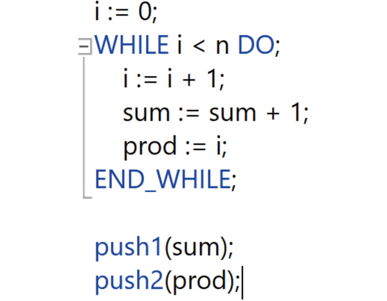
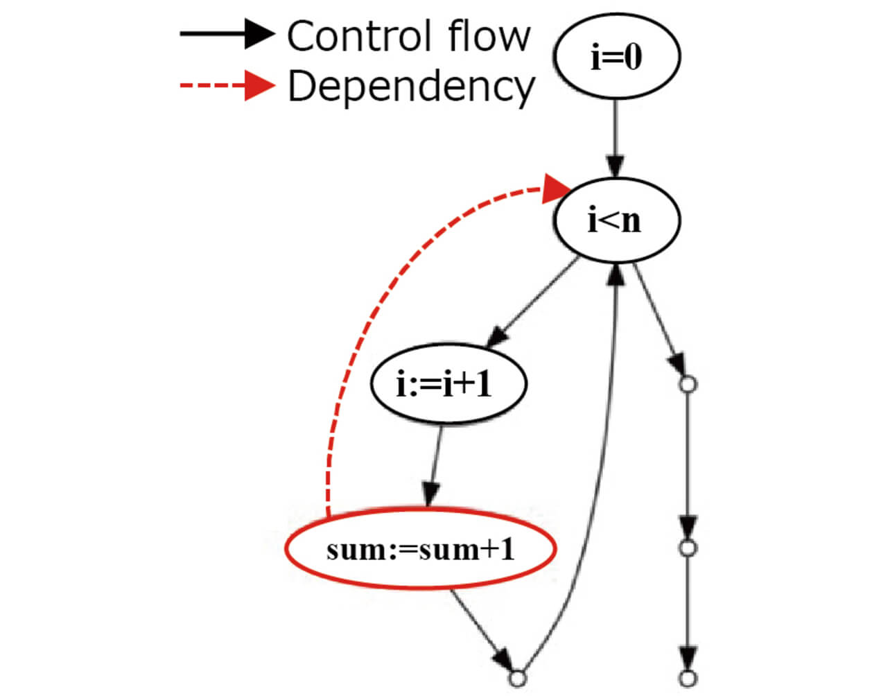
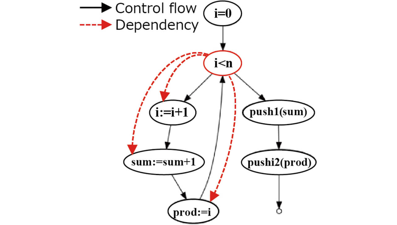
As a result of backward slicing, it turns out that the variables affecting sum are n and i. As a result of forward slicing, the variables affected by n are identified as i, sum, and prod. The variable dependency is expressed as:

which has a value of 1 if var 1 affects var 2; or 0 if not.
3.3 Variable dependence graph
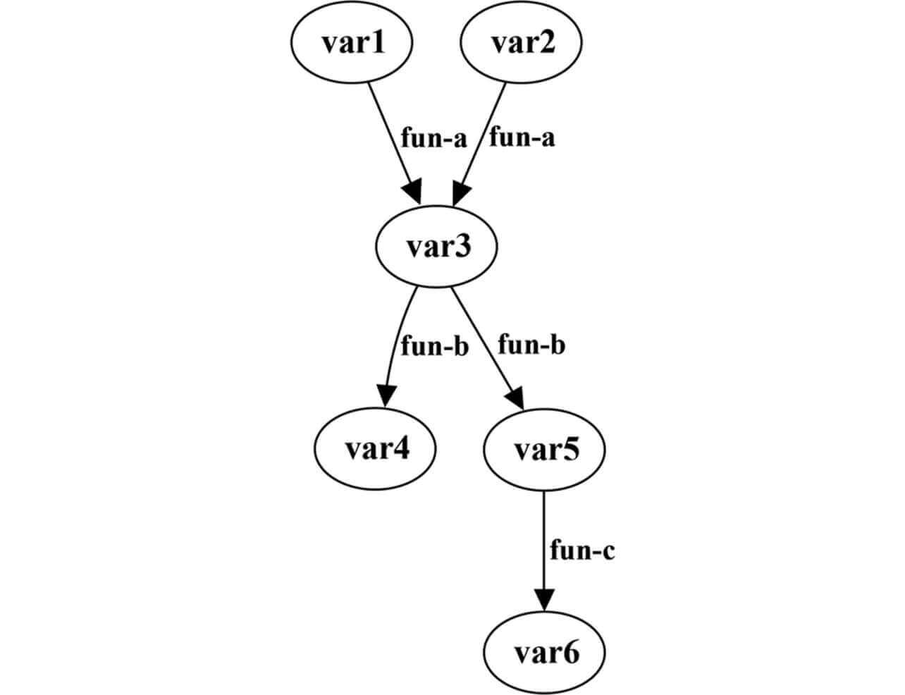
This subsection describes the method of generating a variable dependence graph from each variable dependency obtained by applying program slicing to a PLC control program. The PLC control program discussed here supports IEC 61131-38), the international standard for PLC programming languages. IEC 61131-3 defines three program organization units (POUs): Program (PROG), Function block (FB) with internal status information, and Function (FUN) without internal status information. These POUs are intended to convert programs into structures on a process-by-process or function-by-function basis to enhance the readability and reusability of programs. Fig. 7 shows a typical behavior of the PLC control program. In addition, Fig. 8 shows a typical variable dependence graph representing the relationships among the variables assigned to the devices in the program in Fig. 7 (device variables).
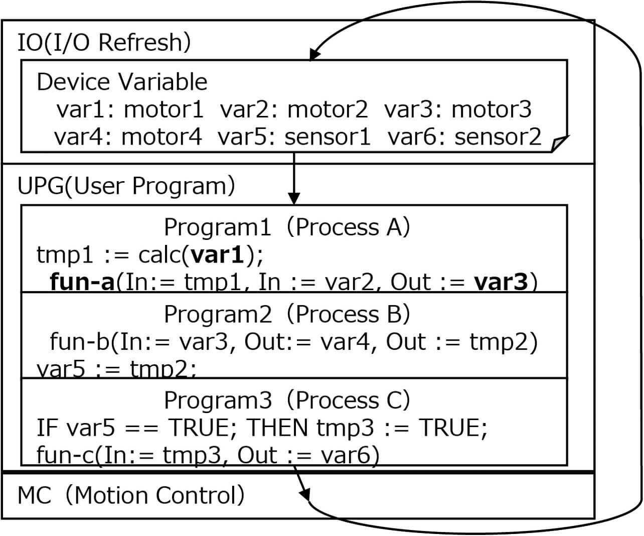
The PLC performs the processing of I/O refresh (Data I/O), user program (UPG) execution, and motion control (MC) tasks at strict time intervals, thereby enabling high-precision control. An I/O refresh task updates device variables assigned to actuators, such as sensors and motors. User programs are executed with device variables as inputs or outputs depending on their process or function.
Our proposed method focuses on a device variable representing a change in the external environment and performs forward slicing to create a dependency between variables. To this dependency, the I/O information to the FB and the FUN, which perform specific processing at each process, is added to generate a variable dependence graph. In Program 1 in Fig. 7, the variable var 1 is entered via tmp 1, the intermediate variable, into fun-a , which then produces var 3 as an output. This flow is also shown by the variable dependence graph in Fig. 8. In the fun-a line, In is the parameter representing the input variable while Out is the parameter representing the output variable.
With the device variables in Fig. 8 given as XN = {var 1, var 2, ... var 6} = {X0, X1, ..., XN–1}, N = 6, the variable dependence graph is expressed by an adjacency matrix given as Eq. (2):

The adjacency matrix is expressed as a square matrix with each variable as a vertex. Dep (Xi , Xj ) is the dependency between the variables given as Expression (1). The variable dependence graph is represented as a directed graph.
3.4 Structural change graph
A control data relationship expression intended to be merged into a variable dependence graph is deemed as a simple structural change detection problem9). A possible approach to this problem is to calculate it by the correlation matrix difference between a normality (nondefective product) and an anomaly (defective product). Pearson’s product-moment correlation coefficient used in general correlation matrices assumes normal distributions. Accordingly, we use a mutual information quantity suitable to express the degree of dependency between time-series control data, such as the one in Fig. 2. This mutual information quantity is expressed as Eq. (3):

Xi and Xj are a pair of control data delimited by the interval required to process the packaging of a single product. The calculation method for the mutual information quantity goes as follows: divide the filled data space in random grids; and, using the maximal information coefficient (MIC)10), search for a grid that maximizes the mutual information quantity.
The mutual information quantity matrix, Amic (XN ), calculated across all the control data is expressed as Eq. (4):

Tables 2 and 3, respectively, show a typical mutual information quantity matrix of normal and anomalous data:
| var1 | var2 | var3 | var4 | var5 | var6 | |
|---|---|---|---|---|---|---|
| var1 | 1.00 | 0.86 | 0.00 | 0.00 | 0.00 | 0.00 |
| var2 | 0.86 | 1.00 | 0.90 | 0.00 | 0.43 | 0.00 |
| var3 | 0.00 | 0.90 | 1.00 | 0.00 | 0.92 | 0.00 |
| var4 | 0.00 | 0.00 | 0.00 | 1.00 | 0.55 | 0.00 |
| var5 | 0.00 | 0.43 | 0.92 | 0.55 | 1.00 | 0.75 |
| var6 | 0.00 | 0.00 | 0.00 | 0.00 | 0.75 | 1.00 |
| var1 | var2 | var3 | var4 | var5 | var6 | |
|---|---|---|---|---|---|---|
| var1 | 1.00 | 0.86 | 0.00 | 0.00 | 0.00 | 0.00 |
| var2 | 0.85 | 1.00 | 0.80 | 0.00 | 0.31 | 0.00 |
| var3 | 0.00 | 0.80 | 1.00 | 0.00 | 0.82 | 0.00 |
| var4 | 0.00 | 0.00 | 0.00 | 1.00 | 0.66 | 0.00 |
| var5 | 0.00 | 0.31 | 0.82 | 0.66 | 1.00 | 0.77 |
| var6 | 0.00 | 0.00 | 0.00 | 0.00 | 0.77 | 1.00 |
Then, the difference in the mutual information quantity between normal and anomalous data is calculated by Eq. (5):

where Amic_normal (XN ) represents normal data and Amic_anormal (XN ) represents anomalous data.
Finally, a structural change graph is calculated from Eq. (6) and represented as in Fig. 9:

With the difference threshold value given as Athreshold (XN ) = 0.05, the step function u is executed once and selects the relationship exceeding the threshold value to generate the structural change graph. Regarding the threshold value, a difference of 0.05 or more in the mutual information quantity is deemed significant based on the five percent level used for permutation tests and the additivity of information quantities11). Note that the structural change graph is undirected and expressed as a symmetric matrix.
3.5 Factor identification graph
A factor identification graph is calculated from Eq. (7) and represented as in Fig. 10:

Eq. (7) uses an Hadamard product, which is an entry-wise matrix product.
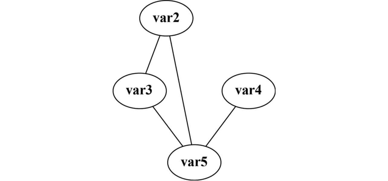
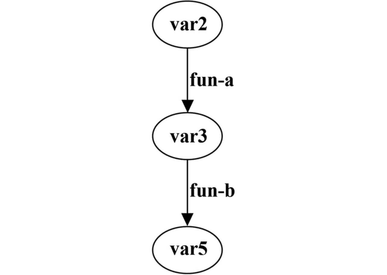
This example shows that the factor is var 2 and affects var 3 via fun-a , whereby var 3, in turn, affects var5 via fun-b . The structural change graph is not represented as a factor identification graph because it exhibits changes in the relationships between var 2 and var 5 and between var 4 and var 5 but shows no relationships found in the variable dependence graph.
4. Verification
This section presents the results of verifying the effectiveness of our proposed method using the experimental packaging machine shown in Subsection 2.1.
4.1 Specifics of the verification
Typical defects observed with packaging machines are packaging defects, the factor of which varies. To verify the effectiveness of our proposed method, we examined two types of packaging defects whose factors cannot be identified by the conventional method. Table 4 shows the outlines of the packaging defects tested here:
| Defect event | Outline | Factor (relevant variable) |
|---|---|---|
| Packaging Defect 1 | A deformed finger led to a misaligned workpiece, resulting in a packaging defect. | Workpiece position error (Conveyor Shaft position) |
| Packaging Defect 2 | The rollers of the film feed shafts went out of parallel and caused film meandering, resulting in a packaging defect. | Film meandering (Film feed shaft 1 velocity, Film feed shaft 2 velocity) |
Packaging Defect 1 was a packaging defect event that resulted from a workpiece position error due to a deformation suffered by a finger for feeding out workpieces. Packaging Defect 2 was a packaging defect event caused by film meandering. The former and the latter had different factors. Then, Table 5 shows a list of collected data used for factor identification:
| Relevant servomotor | Object variable | Control data (unit) |
|---|---|---|
| Film Feed Shaft 1 | FilmFeedMain | FilmFeedMain.Trq (%) FilmFeedMain.Vel (mm/s) FilmFeedMain.Pos (mm) |
| Film Feed Shaft 2 | FilmFeedSub | FilmFeedSub.Trq (%) FilmFeedSub.Vel (mm/s) FilmFeedSub.Pos (mm) |
| Conveyor Shaft | ProductFeed | ProductFeed.Trq (%) ProductFeed.Vel (mm/s) ProductFeed.Pos (mm) |
| Top Seal Shaft | TopSeal | TopSeal.Trq (%) TopSeal.Vel (mm/s) TopSeal.Pos (mm) |
| Virtual Axis | VirtualMaster | N/A |
This table correlates the object variables of the control program with the collected control data for the servomotors constituting parts of the packaging machine. A virtual axis for synchronous control is added to the object variables of the control program. The control data consist of torque (Trq), velocity (Vel), and position (Pos) values, the feedback values of the servo driver that controls the servomotors according to commands from the PLC. Note that each torque value is given as a ratio to the rated torque of 100%. Although each type of control data is in a unit different from the others, no normalization is required because the structural change graph presented in Subsection 3.4 was generated using the MIC.
4.2 Verification results
Fig. 11 shows a variable dependence graph generated by the method presented in Subsection 3.3:
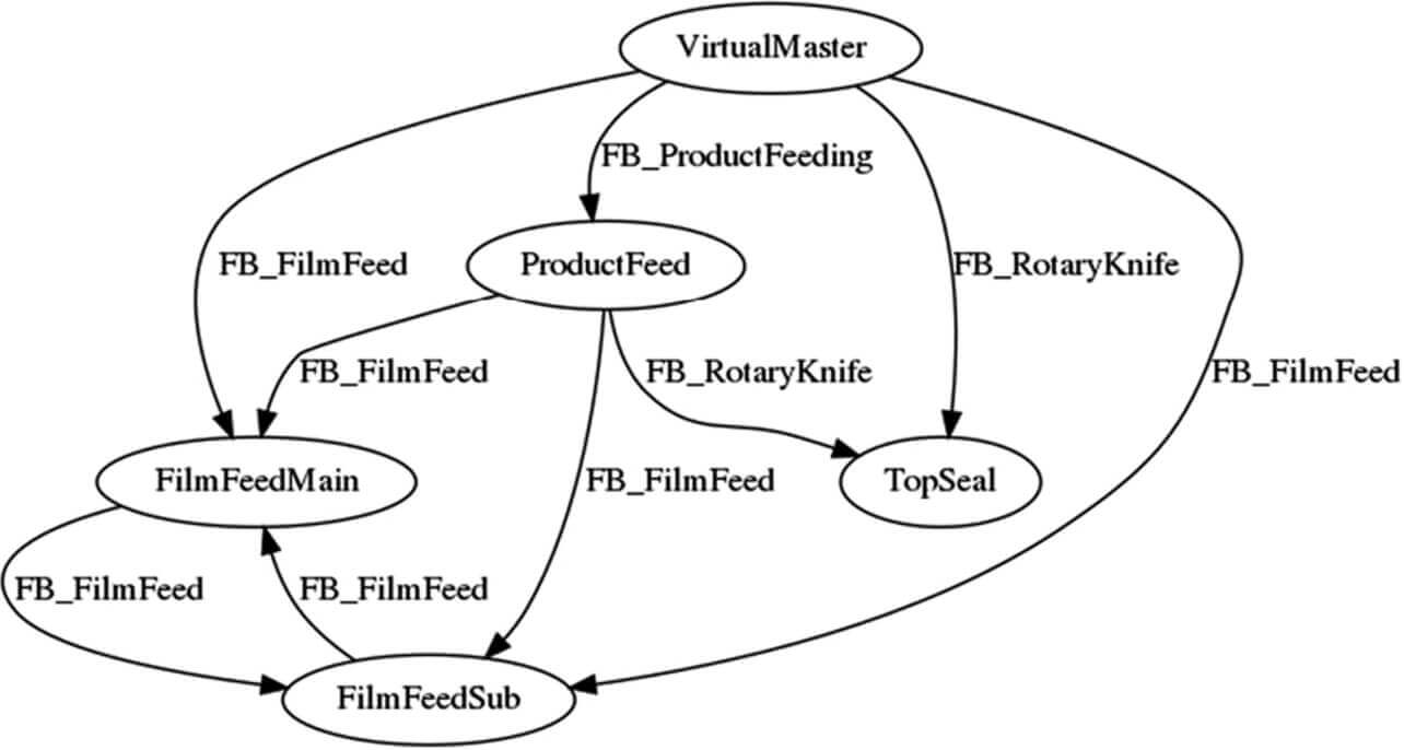
Table 6 correlates the affecting and affected variables based on the variable dependence graph for each FB executed in each process:
| Process | FB | Affecting variable | Affected variable |
|---|---|---|---|
| Workpiece feed process | FB_ProductFeeding | VirtualMaster (Virtual Axis) | ProductFeed (Conveyor Shaft) |
| Center seal process | FB_FilmFeed | VirtualMaster (Virtual Axis) ProductFeed (Conveyor Shaft) FilmFeedMain (Film Feed Shaft 1) FilmFeedSub (Film Feed Shaft 2) |
FilmFeedMain (Film Feed Shaft 1) FilmFeedSub (Film Feed Shaft 2) |
| End seal process | FB_RotaryKnife | VirtualMaster (Virtual Axis) ProductFeed (Conveyor Shaft) |
TopSeal (Top Seal Shaft) |
In the center seal process, film feed shafts 1 and 2 affect each other, turning out to be in a circular relationship.
Then, Table 7 shows the mutual information quantity matrix calculated by the method presented in Subsection 3.4 for the control data for a product in a nondefective condition.
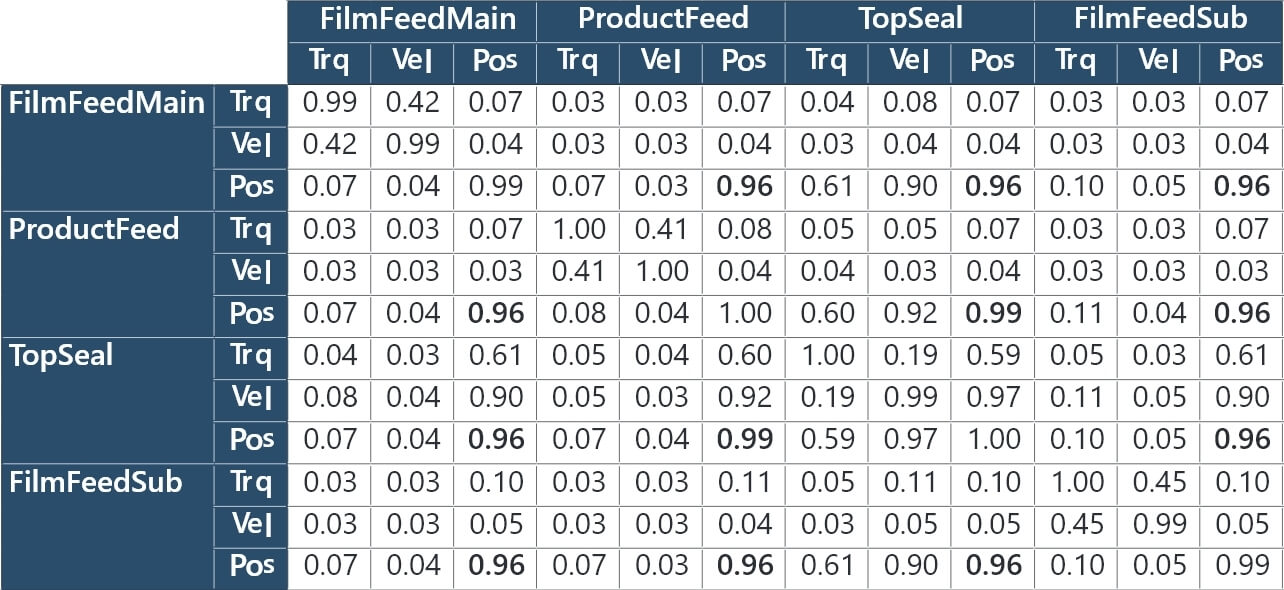
The FilmFeedMain, ProductFeed, TopSeal, and FilmFeedSub positions (Pos) all show high relationship scores (0.95 or more). These results are because the packaging machine synchronously controls these positions based on ProductFeed for workpiece conveyance. These results show that the FilmFeedMain, ProductFeed, TopSeal, and FilmFeedSub positions can all be consolidated into the ProductFeed position upstream in the variable dependence graph in Fig. 11.
Similarly, Table 8 shows the differences in the mutual information quantity matrix between the non-defective product and Packaging Defect 1 as calculated by the method presented in Subsection 3.4.
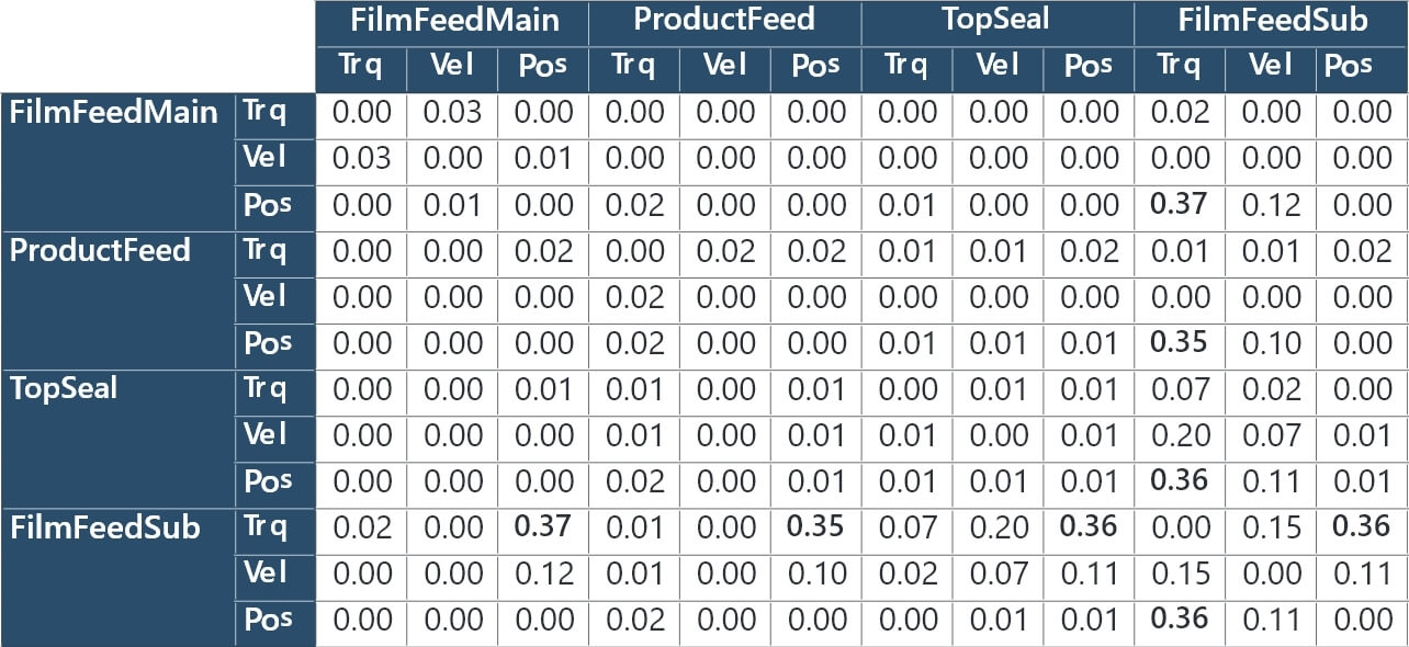
Fig. 12 shows a structural change graph generated with a threshold value of 0.32 based on these results. This graph has torques and other elements indicated on its edges for the convenience of merging with the variable dependence graph. Fig. 13 is a modified version of this graph with all its position information consolidated, as explained above, into ProductFeed.


Finally, Fig. 14 shows a factor identification graph generated by the method presented in Subsection 3.5.
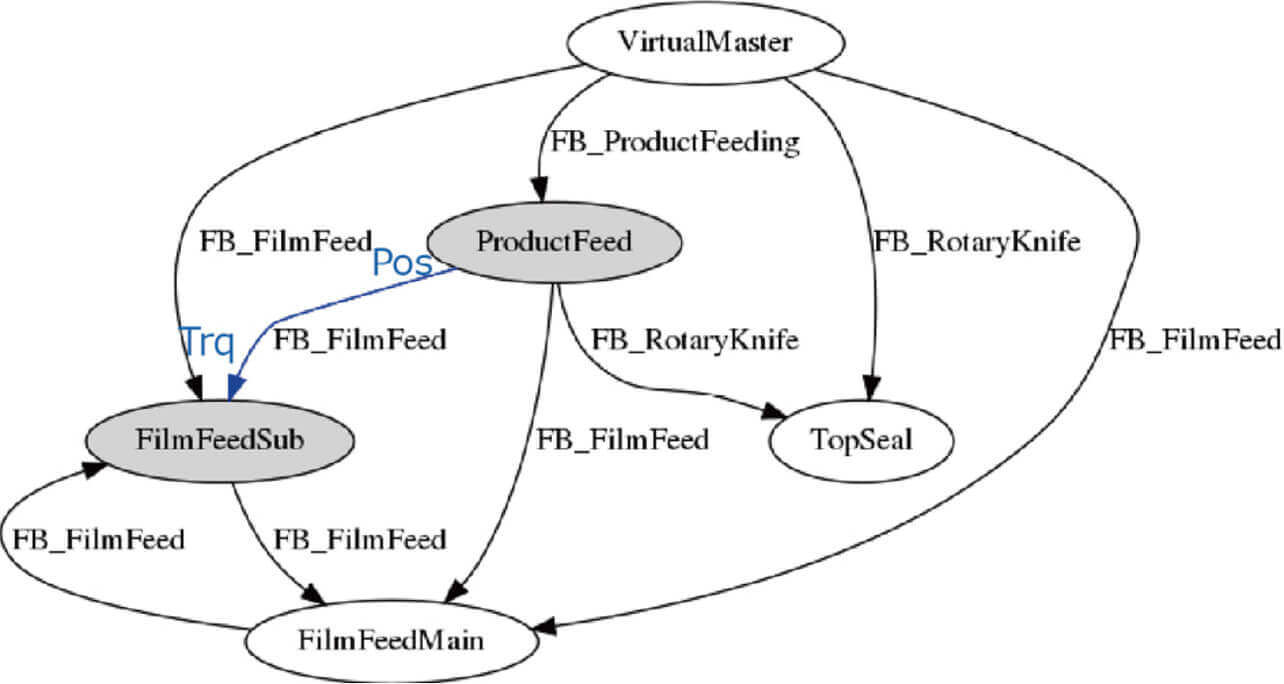
As a result, the position information of ProductFeed serving the workpiece feed process was identified as the cause and found consistent with the Conveyor Shaft position, the factor. Then, Fig. 15 shows a factor identification graph generated by the same method for Packaging Defect 2:
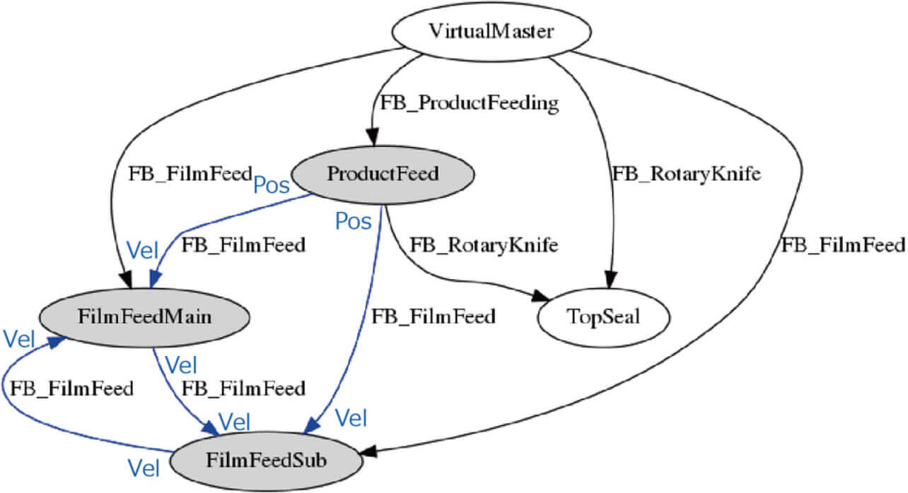
Two potential factors are assumed here: a ProductFeed position value affecting the FilmFeedMain/Sub velocity and a collapse of the FilmFeedMain/Sub velocity relationship. This defect factor is film meandering. The collapse of the velocity relationship between FilmFeedMain and FilmFeedSub, which are film feed shafts 1 and 2, is consistent with the factor. Table 9 summarizes the factor identification results by our proposed method. This table adds the factor identification results by our proposed method and the conventional method to the defect types and factors shown in Table 4.
| Defect type | Factor | Factor identification results by our proposed method | Factor identification results by the conventional method | Importance |
|---|---|---|---|---|
| Packaging Defect 1 | Workpiece position error (Conveyor shaft position) |
Conveyor shaft position | Film feed shaft 2 torque (standard deviation) | 0.154 |
| Film feed shaft 2 velocity (max) | 0.137 | |||
| Top Seal Shaft torque (min) | 0.081 | |||
| Conveyor shaft position (standard deviation) | 0.007 | |||
| Packaging Defect 2 | Film meandering (Film feed shaft 1 velocity, film feed shaft 2 velocity) |
Conveyor shaft position Collapse of velocity relationship between film feed shafts 1 and 2 |
Film feed shaft 1 torque (mean) | 0.169 |
| Top seal shaft torque (min) | 0.123 | |||
| Top seal shaft velocity (min) | 0.120 | |||
| Film feed shaft 1 velocity (mean) | 0.016 | |||
| Film feed shaft 2 velocity (mean) | 0.031 |
For Packaging Defect 1, our proposed method successfully identified the factor as intended. For Packaging Defect 2, it narrowed down potential factors to two. For the conventional method, Table 9 shows the top three feature quantities calculated based on RandomForest importance values and the importance values of the feature quantities corresponding to the true factor similarly to Subsection 2.3. The feature quantities identified by the conventional method showed higher importance values than that of the true factor and turned out to be unsuitable for factor identification.
4.3 Discussion
This subsection discusses the respective validity of the mutual information quantity matrix and factor identification for configuring the variable dependency and structural change graphs. The variable dependence graph has successfully extracted the intended process information and represented the relationships among variables. The mutual information quantity matrix generated exclusively from the non-defective product data clearly represents the synchronous control of the servomotor position, suggesting that the obtained results are highly plausible from a control perspective.
Our proposed method correctly identified the position information of the conveyor shaft, which serves as the workpiece feed process, as the factor for Packaging Defect 1. For Packaging Defect 2, our proposed method narrowed down potential factors to two: the position information of the conveyor shaft and the velocity relationship between film feed shafts 1 and 2. Unlike the conventional method, which showed a tendency to identify factors in the downstream process, our proposed method identified a true factor, suggesting its effectiveness in factor identification.
On the other hand, however, our proposed method failed to identify down to a single factor for Packaging Defect 2 and picked the conveyor shaft position. A possible cause may be that this method focuses on data relationships and accordingly ends up extracting both halves of an edge when a change occurs only in either half. Moving forward, we need to consider making improvements, such as adding the importance values of feature quantities to data relationships.
One more point to add is that while we applied our proposed method to a relatively small-scale system consisting of four servomotors, large-scale systems consisting of around 100 servomotors would also come into the scope of application of our proposed method to production lines. Our proposed method can generate factor identification graphs for large-scale systems. However, its application to a system with around more than 20 servomotors would result in a complicated factor identification graph, posing an interpretability issue. This point will be addressed in the future.
5. Conclusions
Aiming to identify defect factors on shop floors in the FA field, we proposed applying a program slicing technique to the problem with data of low independence due to multiple synchronized processes, extracting knowledge information from a PLC control program containing multi-processing and synchronous control information, and integrating the extracted knowledge information into data analysis. In an effectiveness verification test using an experimental packaging machine, we demonstrated the effectiveness of our proposed method in identifying factors unidentifiable by the conventional method. Besides, our proposed method extracts knowledge information from the PLC control program and can be implemented without checking the real program, thereby reducing the man-hours needed for factor analysis.
Regarding the future prospects for our proposed method, we will work on its issues with data relationship accuracy improvement and applicability to large-scale systems and would also like to expand its scope of applicability by adapting the targeted control program to PLCs of other makes or extracting knowledge information from design documents and other sources other than the program.
References
- 1)
- Toshiba Corporation, “HMLasso™ Factor Analysis Technology,” (in Japanese), in Toshiba AI Technology Catalog, Apr. 1, 2020, https://www.global.toshiba/jp/technology/corporate/ai/catalog013.html (accessed Mar. 1, 2022).
- 2)
- NEC Corporation, “Quality Control in Manufacturing Plants Using a Factor Analysis Engine,” (in Japanese), NEC Tech. Rep., Sep. 2016, https://jpn.nec.com/techrep/journal/g16/n01/160114.html (accessed Mar. 1, 2022).
- 3)
- K. Ishikawa, Introduction to Quality Control, 3rd Ed. (in Japanese), Tokyo, JUSE Press, Ltd., 1989.
- 4)
- K. Tsuruta, T. Minemoto, and Y. Hirohashi, “Development of AI Technology for Machine Automation Controller (1),” (in Japanese), OMRON TECHNICS, vol. 50, no. 1, pp. 6-11, 2018.
- 5)
- K. Miyamoto and S. Kawanoue, “Development of AI-equipped Machine Automation Controller (3),” (in Japanese), OMRON TECHNICS, vol. 51, no. 1, pp. 52-57, 2019.
- 6)
- Productivity Press Development Team, OEE for Operators: Overall Equipment Effectiveness, 1st Ed., Productivity Press, 2018.
- 7)
- D. W. Binkley and K. B. Gallagher, “Program Slicing,” Adv. Comput., vol. 43, pp. 1-50, 1996.
- 8)
- OMRON Corporation, “International Standard Programming for PLCs: What is IEC 61131-3?” (in Japanese), Sysmac Integrated Platform, https://www.fa.omron.co.jp/product/special/sysmac/plcopen/feature1.html (accessed Mar. 1, 2022).
- 9)
- T. Ide and M. Sugiyama, Anomaly Detection and Change Detection (in Japanese), Tokyo, Kodansha Ltd., 2015, p.162.
- 10)
- D. N. Reshef, et al., “Detecting Novel Associations in Large Data Sets,” Science, vol. 334, no. 6062, pp. 1518-1524, 2011.
- 11)
- M. Sugiyama, K. Irie, and M. Tomono, “Machine Learning with Mutual Information and Its Application in Robotics,” (in Japanese), J. Rob. Soc. Jpn, vol. 33, no. 2, pp. 86-91, 2015.
The names of products in the text may be trademarks of each company.